Main Content

structuralBC

Specify boundary conditions for structural model

Description

Standard Boundary Constraints and Displacements

example

structuralBC(structuralmodel,RegionType,RegionID,"Constraint",Cval) specifies one of the standard structural boundary constraints. Here, Cval can be "fixed", "free", "roller", or "symmetric". The default value is "free".

Avoid using "symmetric" for transient and modal analysis, since the symmetric constraint can prevent the participation of some structural modes.

example

structuralBC(structuralmodel,RegionType,RegionID,"Displacement",Dval) enforces displacement on the boundary of type RegionType with RegionID ID numbers.

example

structuralBC(structuralmodel,RegionType,RegionID,"XDisplacement",XDval,"YDisplacement",YDval,"ZDisplacement",ZDval) specifies the x-, y-, and z-components of the enforced displacement.

structuralBC does not require you to specify all three components. Depending on your structural analysis problem, you can specify one or more components by picking the corresponding arguments and omitting others.

example

structuralBC(structuralmodel,RegionType,RegionID,"RDisplacement",RDval,"ZDisplacement",ZDval) specifies the r- and z-components of the enforced displacement for an axisymmetric model. The radial component (r-component) must be zero on the axis of rotation.

structuralBC does not require you to specify both components.

Harmonic, Rectangular, Triangular, and Trapezoidal Displacement Pulses

example

structuralBC(structuralmodel,RegionType,RegionID,"XDisplacement",XDval,Name,Value)specifies the form and duration of the time-varying value of the x-component of the enforced displacement. You can also specify the form and duration of the other components of the displacement as follows:

  • structuralBC(...,"YDisplacement",YDval,Name,Value) for the y-component.

  • structuralBC(...,"ZDisplacement",ZDval,Name,Value) for the z-component. Use this syntax for a 3-D or axisymmetric model.

  • structuralBC(...,"RDisplacement",RDval,Name,Value) for the radial component in an axisymmetric model.

Multipoint Constraint

example

structuralBC(structuralmodel,RegionType,RegionID,"Constraint","multipoint") sets the multipoint constraint using all degrees of freedom on the combination of geometric regions specified by RegionType and RegionID. The reference location for the constraint is the geometric center of all nodes on the combination of all specified geometric regions.

This syntax is required if you intend to use results obtained with the model order reduction technique in the Simscape™ Multibody™ Reduced Order Flexible Solid block. Simscape models expect the connections at all joints to have six degrees of freedom, while Partial Differential Equation Toolbox™ uses two or three degrees of freedom at each node. Setting a multipoint constraint ensures that all nodes and all degrees of freedom for the specified geometric regions have a rigid constraint with the geometric center of all specified geometric regions altogether as the reference point. The reference location has six degrees of freedom.

For better performance, specify geometric regions with a minimal number of nodes. For example, use a set of edges instead of using a face, and a set of vertices instead of using an edge.

structuralBC(___,"Reference",Coords) specifies the reference point for the multipoint constraint instead of using the geometric center of all specified regions as a reference point.

Use this syntax with the input arguments from the previous syntax.

structuralBC(___,"Reference",Coords,"Radius",R) restricts the region for multipoint constraint to nodes within the circle (for a 2-D geometry) or sphere (for a 3-D geometry) of radius R around the reference point.

Sparse Linear Models for Use with Control System Toolbox

structuralBC(___,"Label",labeltext) adds a label for the structural boundary condition to be used by the linearizeInput function. This function lets you pass boundary conditions to the linearize function that extracts sparse linear models for use with Control System Toolbox™.

Vectorized Evaluation for Function Handles

structuralBC(___,"Vectorized","on") uses vectorized function evaluation when you pass a function handle as an argument. If your function handle computes in a vectorized fashion, then using this argument saves time. See Vectorization. For details on this evaluation, see Nonconstant Boundary Conditions.

Use this syntax with any of the input arguments from previous syntaxes.

Structural Boundary Condition Object

bc = structuralBC(___) returns the structural boundary condition object using any of the input arguments from previous syntaxes.

Examples

collapse all

Apply fixed boundaries and traction on two ends of a bimetallic cable.

Create a structural model.

structuralModel = createpde("structural","static-solid");

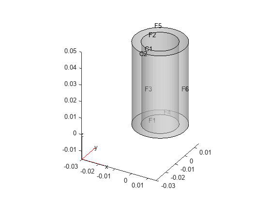
Create nested cylinders to model a bimetallic cable.

gm = multicylinder([0.01,0.015],0.05);

Assign the geometry to the structural model and plot the geometry.

structuralModel.Geometry = gm;
pdegplot(structuralModel,"CellLabels","on", ...
                         "FaceLabels","on", ...
                         "FaceAlpha",0.4)

For each metal, specify Young's modulus and Poisson's ratio.

structuralProperties(structuralModel,"Cell",1,"YoungsModulus",110E9, ...
                                              "PoissonsRatio",0.28);
structuralProperties(structuralModel,"Cell",2,"YoungsModulus",210E9, ...
                                              "PoissonsRatio",0.3);

Specify that faces 1 and 4 are fixed boundaries.

structuralBC(structuralModel,"Face",[1,4],"Constraint","fixed")
ans = 
  StructuralBC with properties:

                RegionType: 'Face'
                  RegionID: [1 4]
                Vectorized: 'off'

   Boundary Constraints and Enforced Displacements
              Displacement: []
             XDisplacement: []
             YDisplacement: []
             ZDisplacement: []
                Constraint: "fixed"
                    Radius: []
                 Reference: []
                     Label: []

   Boundary Loads
                     Force: []
           SurfaceTraction: []
                  Pressure: []
    TranslationalStiffness: []
                     Label: []

Specify the surface traction for faces 2 and 5.

structuralBoundaryLoad(structuralModel, ...
                          "Face",[2,5], ...
                          "SurfaceTraction",[0;0;100])
ans = 
  StructuralBC with properties:

                RegionType: 'Face'
                  RegionID: [2 5]
                Vectorized: 'off'

   Boundary Constraints and Enforced Displacements
              Displacement: []
             XDisplacement: []
             YDisplacement: []
             ZDisplacement: []
                Constraint: []
                    Radius: []
                 Reference: []
                     Label: []

   Boundary Loads
                     Force: []
           SurfaceTraction: [3x1 double]
                  Pressure: []
    TranslationalStiffness: []
                     Label: []

Create a structural model.

structuralModel = createpde("structural","static-solid");

Create a block geometry.

gm = multicuboid(0.2,0.1,0.05);

Assign the geometry to the structural model and plot the geometry.

structuralModel.Geometry = gm;
pdegplot(structuralModel,"FaceLabels","on","FaceAlpha",0.5)

Specify Young's modulus, Poisson's ratio, and the mass density.

structuralProperties(structuralModel,"YoungsModulus",74e9,...
                                     "PoissonsRatio",0.42,...
                                     "MassDensity",19.29e3);

Specify the gravity load on the beam.

structuralBodyLoad(structuralModel, ...
    "GravitationalAcceleration",[0;0;-9.8]);

Specify that face 5 is a fixed boundary.

structuralBC(structuralModel,"Face",5,"Constraint","fixed");

Specify z-displacement on face 3 of the model. By leaving the x- and y-displacements unspecified, you enable face 3 to move in the x- and y-directions.

structuralBC(structuralModel,"Face",3,"ZDisplacement",0.0001);

Generate a mesh and solve the model.

generateMesh(structuralModel);
R = solve(structuralModel); 

Plot the deformed shape with the x-component of normal stress.

pdeplot3D(structuralModel,"ColorMapData",R.Stress.sxx, ...
                          "Deformation",R.Displacement)

Now specify all three displacements on the same face. Here, the z-displacement is the same, but the x- and y-displacements are both zero. Face 3 cannot move in the x- and y-directions.

structuralBC(structuralModel,"Face",3, ...
                             "Displacement",[0;0;0.0001]); 
R = solve(structuralModel);
pdeplot3D(structuralModel,"ColorMapData",R.Stress.sxx, ...
                          "Deformation",R.Displacement)

Thus, specifying "Displacement",[0;0;0.0001] is equivalent to specifying "XDisplacement",0,"YDisplacement",0,"ZDisplacement",0.0001.

structuralBC(structuralModel,"Face",3,"XDisplacement",0, ...
                                      "YDisplacement",0, ...
                                      "ZDisplacement",0.0001); 
R = solve(structuralModel);
pdeplot3D(structuralModel,"ColorMapData",R.Stress.sxx, ...
                          "Deformation",R.Displacement)

Analyze a spinning disk with radial compression at the hub due to press-fit. The inner radius of the disk is 0.05, and the outer radius is 0.2. The thickness of the disk is 0.05 with an interference fit of 50E-6. For this analysis, simplify the 3-D axisymmetric model to a 2-D model.

Create a static structural analysis model for solving an axisymmetric problem.

structuralmodel = createpde("structural","static-axisymmetric");

The 2-D model is a rectangular strip whose x-dimension extends from the hub to the outer surface, and whose y-dimension extends over the height of the disk. Create the geometry by specifying the coordinates of the strip's four corners. For axisymmetric models, the toolbox assumes that the axis of rotation is the vertical axis passing through r = 0, which is equivalent to x = 0.

g = decsg([3 4 0.05 0.2 0.2 0.05 -0.025 -0.025 0.025 0.025]');

Include the geometry in the model.

geometryFromEdges(structuralmodel,g);

Plot the geometry with the edge and vertex labels.

figure
pdegplot(structuralmodel,"EdgeLabels","on","VertexLabels","on")
xlim([0 0.3])
ylim([-0.05 0.05])

Specify Young's modulus, Poisson's ratio, and the mass density.

structuralProperties(structuralmodel,"YoungsModulus",210e9, ...
                                     "PoissonsRatio",0.28, ...
                                     "MassDensity",7700);

Apply centrifugal load due to spinning of the disk. Assume that the disk is spinning at 104.7 rad/s.

structuralBodyLoad(structuralmodel,"AngularVelocity",104.7);

Apply radial displacement at the hub of the disk to model press-fit.

structuralBC(structuralmodel,"Edge",4,"RDisplacement",50e-6);

Fix axial displacement of a point on the hub to prevent rigid body motion.

structuralBC(structuralmodel,"Vertex",1,"ZDisplacement",0);

Generate a mesh.

generateMesh(structuralmodel);

Solve the model.

structuralresults = solve(structuralmodel);

Plot the radial displacement of the disk.

figure
pdeplot(structuralmodel, ...
        "XYData",structuralresults.Displacement.ur, ...
        "ColorMap","jet")
axis equal
xlim([0 0.3])
ylim([-0.05 0.05])

Plot circumferential (hoop) stress.

figure
pdeplot(structuralmodel, ...
        "XYData",structuralresults.Stress.sh, ...
        "ColorMap","jet")
axis equal
xlim([0 0.3])
ylim([-0.05 0.05])

Use a function handle to specify a harmonically varying excitation in a beam.

Create a transient dynamic model for a 3-D problem.

structuralmodel = createpde("structural","transient-solid");

Create a geometry and include it in the model. Plot the geometry.

gm = multicuboid(0.06,0.005,0.01);
structuralmodel.Geometry = gm;
pdegplot(structuralmodel,"FaceLabels","on","FaceAlpha",0.5)
view(50,20)

Specify Young's modulus, Poisson's ratio, and the mass density of the material.

structuralProperties(structuralmodel,"YoungsModulus",210E9, ...
                                     "PoissonsRatio",0.3, ...
                                     "MassDensity",7800);

Fix one end of the beam.

structuralBC(structuralmodel,"Face",5,"Constraint","fixed");

Apply a sinusoidal displacement along the y-direction on the end opposite to the fixed end of the beam.

yDisplacementFunc = ...
@(location,state) ones(size(location.y))*1E-4*sin(50*state.time);
structuralBC(structuralmodel,"Face",3, ...
                             "YDisplacement",yDisplacementFunc);

Specify a harmonically varying excitation by specifying its frequency.

Create a transient dynamic model for a 3-D problem.

structuralmodel = createpde("structural","transient-solid");

Create a geometry and include it in the model. Plot the geometry.

gm = multicuboid(0.06,0.005,0.01);
structuralmodel.Geometry = gm;
pdegplot(structuralmodel,"FaceLabels","on","FaceAlpha",0.5)
view(50,20)

Specify Young's modulus, Poisson's ratio, and the mass density of the material.

structuralProperties(structuralmodel,"YoungsModulus",210E9, ...
                                     "PoissonsRatio",0.3, ...
                                     "MassDensity",7800);

Fix one end of the beam.

structuralBC(structuralmodel,"Face",5,"Constraint","fixed");

Apply a sinusoidal displacement along the y-direction on the end opposite to the fixed end of the beam.

structuralBC(structuralmodel,"Face",3, ...
                             "YDisplacement",1E-4, ...
                             "Frequency",50);

Fix one corner of a rectangular plate to restrain all rigid body motions of the model.

Create a structural model for static plane-stress analysis.

model = createpde("structural","static-planestress"); 

Create the geometry and include it in the structural model.

length = 1;
width = 0.5;
radius = 0.1;
R1 = [3 4 -length length length -length ...
          -width -width  width   width]';
C1 = [1 0 0 radius 0 0 0 0 0 0]';
gdm = [R1 C1];
ns = char('R1','C1');
g = decsg(gdm,'R1- C1',ns');
geometryFromEdges(model,g);

Plot the geometry, displaying edge labels.

figure
pdegplot(model,"EdgeLabels","on");
axis([-1.2*length 1.2*length ...
      -1.2*width  1.2*width])

Plot the geometry, displaying vertex labels.

figure
pdegplot(model,"VertexLabels","on");
axis([-1.2*length 1.2*length ...
      -1.2*width  1.2*width])

Specify Young's modulus and Poisson's ratio of the material.

structuralProperties(model,"YoungsModulus",210E9,"PoissonsRatio",0.3);

Set the x-component of displacement on the left edge of the plate to zero to resist the applied load.

structuralBC(model,"Edge",3,"XDisplacement",0);

Apply the surface traction with a nonzero x-component on the right edge of the plate.

structuralBoundaryLoad(model,"Edge",1,"SurfaceTraction",[100000 0]);

Set the y-component of displacement at the bottom-left corner (vertex 3) to zero to restraint the rigid body motion.

structuralBC(model,"Vertex",3,"YDisplacement",0);

Generate the mesh, using Hmax to control the mesh size. A fine mesh lets you capture the gradation in the solution accurately.

generateMesh(model,"Hmax",radius/6);

Solve the problem.

R = solve(model); 

Plot the x-component of the normal stress distribution.

pdeplot(model,"XYData",R.Stress.sxx);
axis equal
colormap jet
title("Normal Stress Along x-Direction")

Set multipoint constraints on two opposite sides of a beam.

Create a transient structural model for a 3-D problem.

structuralmodel = createpde("structural","transient-solid");

Create a geometry and include it in the model. Plot the geometry.

gm = multicuboid(0.1,0.01,0.01);
structuralmodel.Geometry = gm;
pdegplot(structuralmodel,"EdgeLabels","on","FaceAlpha",0.5)

Specify Young's modulus, Poisson's ratio, and the mass density of the material.

structuralProperties(structuralmodel,"YoungsModulus",70E9, ...
                                     "PoissonsRatio",0.3, ...
                                     "MassDensity",2700);

Generate a mesh.

generateMesh(structuralmodel);

Set the multipoint constraint on the right side of the beam. For better performance, set the constraint on the set of edges bounding the right side of the beam instead of setting it on the entire face.

structuralBC(structuralmodel,"Edge",[4,6,9,10], ...
                             "Constraint","multipoint")
ans = 
  StructuralBC with properties:

                RegionType: 'Edge'
                  RegionID: [4 6 9 10]
                Vectorized: 'off'

   Boundary Constraints and Enforced Displacements
              Displacement: []
             XDisplacement: []
             YDisplacement: []
             ZDisplacement: []
                Constraint: "multipoint"
                    Radius: []
                 Reference: []
                     Label: []

   Boundary Loads
                     Force: []
           SurfaceTraction: []
                  Pressure: []
    TranslationalStiffness: []
                     Label: []

   Time Variation of Force, Pressure, or Enforced Displacement
                 StartTime: []
                   EndTime: []
                  RiseTime: []
                  FallTime: []

   Sinusoidal Variation of Force, Pressure, or Enforced Displacement
                 Frequency: []
                     Phase: []

Using the same approach, set the multipoint constraint on the left side of the beam.

structuralBC(structuralmodel,"Edge",[2,8,11,12], ...
                             "Constraint","multipoint")
ans = 
  StructuralBC with properties:

                RegionType: 'Edge'
                  RegionID: [2 8 11 12]
                Vectorized: 'off'

   Boundary Constraints and Enforced Displacements
              Displacement: []
             XDisplacement: []
             YDisplacement: []
             ZDisplacement: []
                Constraint: "multipoint"
                    Radius: []
                 Reference: []
                     Label: []

   Boundary Loads
                     Force: []
           SurfaceTraction: []
                  Pressure: []
    TranslationalStiffness: []
                     Label: []

   Time Variation of Force, Pressure, or Enforced Displacement
                 StartTime: []
                   EndTime: []
                  RiseTime: []
                  FallTime: []

   Sinusoidal Variation of Force, Pressure, or Enforced Displacement
                 Frequency: []
                     Phase: []

Reduce the model to all modes in the frequency range [-Inf,500000] and the interface degrees of freedom.

R = reduce(structuralmodel,"FrequencyRange",[-Inf,500000]);

Input Arguments

collapse all

Structural model, specified as a StructuralModel object. The model contains the geometry, mesh, structural properties of the material, body loads, boundary loads, and boundary conditions.

Example: structuralmodel = createpde("structural","transient-solid")

Geometric region type, specified as "Vertex", "Edge", or, for a 3-D model, "Face".

You cannot use the following geometric region types if you specify the "roller" or "symmetric" value for the boundary constraint Cval:

  • "Edge" for a 3-D model

  • "Vertex" for a 2-D or 3-D model

Example: structuralBC(structuralmodel,"Face",[2,5],"XDisplacement",0.1)

Data Types: char | string

Geometric region ID, specified as a vector of positive integers. Find the region IDs by using pdegplot.

Example: structuralBC(structuralmodel,"Face",[2,5],"XDisplacement",0.01)

Data Types: double

Displacement

Enforced displacement, specified as a numeric vector or function handle. A numeric vector must contain two elements for a 2-D model (including axisymmetric models) and three elements for a 3-D model. The function must return a two-row matrix for a 2-D model and a three-row matrix for a 3-D model. Each column of the matrix must correspond to an enforced displacement vector at the boundary coordinates provided by the solver. In case of a transient or frequency response analysis, Dval also can be a function of time or frequency, respectively. For details, see More About.

Note that when you specify Dval for an axisymmetric model, the radial displacement on the axis of rotation must always be zero.

Example: structuralBC(structuralmodel,"Face",[2,5],"Displacement",[0;0;0.01])

Data Types: double | function_handle

x-component of enforced displacement, specified as a number or function handle. The function must return a row vector. Each element of this vector corresponds to the x-component value of the enforced displacement at the boundary coordinates provided by the solver. In case of a transient or frequency response analysis, XDval also can be a function of time or frequency, respectively. For details, see More About.

Example: structuralBC(structuralmodel,"Face",[2,5],"XDisplacement",0.01)

Data Types: double | function_handle

y-component of enforced displacement, specified as a number or function handle. The function must return a row vector. Each element of this vector corresponds to the y-component value of the enforced displacement at the boundary coordinates provided by the solver. In case of a transient or frequency response analysis, YDval also can be a function of time or frequency, respectively. For details, see More About.

Example: structuralBC(structuralmodel,"Face",[2,5],"YDisplacement",0.01)

Data Types: double | function_handle

z-component of enforced displacement, specified as a number or function handle. The function must return a row vector. Each element of this vector corresponds to the z-component value of the enforced displacement at the boundary coordinates provided by the solver. For a transient or frequency response analysis, ZDval also can be a function of time or frequency, respectively. For details, see More About.

You can specify ZDval for a 3-D or axisymmetric model.

Example: structuralBC(structuralmodel,"Face",[2,5],"ZDisplacement",0.01)

Data Types: double | function_handle

r-component of enforced displacement, specified as a number or function handle. The function must return a row vector. Each element of this vector corresponds to the r-component value of the enforced displacement at the boundary coordinates provided by the solver. For a transient or frequency response analysis, RDval also can be a function of time or frequency, respectively. For details, see More About.

You can specify RDval only for an axisymmetric model. RDval must be zero on the axis of rotation.

Example: structuralBC(structuralmodel,"Face",[2,5],"RDisplacement",0.01)

Data Types: double | function_handle

Standard structural boundary constraints, specified as "free","fixed","roller", "symmetric", or "multipoint".

You cannot use the "roller" and "symmetric" values with the following geometric region types:

  • "Edge" for a 3-D model

  • "Vertex" for a 2-D or 3-D model

Example: structuralBC(structuralmodel,"Face",[2,5],"Constraint","fixed")

Data Types: char | string

Reference point location for the multipoint constraint, specified as a 2-by-1 (for a 2-D geometry) or 3-by-1 (for a 3-D geometry) numeric vector.

Example: structuralBC(structuralmodel,"Vertex",[1,3,5:10],"Constraint","multipoint","Reference",[0;0;1])

Data Types: double

Radius of a circle (for a 2-D geometry) or a sphere (for a 3-D geometry) around the reference point location for the multipoint constraint, specified as a positive number.

Example: structuralBC(structuralmodel,"Vertex",[1,3,5:10],"Constraint","multipoint","Reference",[0;0;1],"Radius",0.2)

Data Types: double

Label for the structural boundary condition, specified as a character vector or a string.

Data Types: char | string

Name-Value Arguments

Example: structuralBC(structuralmodel,"Face",[2,5],"XDisplacement",0.01,"RiseTime",0.5,"FallTime",0.5,"EndTime",3)

Use one or more name-value pair arguments to specify the form and duration of the time-varying value of a component of displacement. Specify the displacement value using one of the following arguments: XDval, YDval, ZDval, or RDval. You cannot use these name-value pair arguments to specify more than one time-varying component or to specify the Dval value.

You can model rectangular, triangular, and trapezoidal displacement pulses. If the start time is 0, you do not need to specify it.

  • For a rectangular pulse, specify the start and end times.

  • For a triangular pulse, specify the start time and any two of the following times: rise time, fall time, and end time. You also can specify all three times, but they must be consistent.

  • For a trapezoidal pulse, specify all four times.

Trapezoidal pulse showing the start, rise, fall, and end times

You can model a harmonic displacement by specifying its frequency and initial phase. If the initial phase is 0, you do not need to specify it.

Harmonic displacement showing the frequency and the initial phase

Rectangular, Triangular, or Trapezoidal Pulse

collapse all

Start time for the displacement component, specified as 0 or a positive number. Specify this argument only for transient structural models.

Example: structuralBC(structuralmodel,"Face",[2,5],"XDisplacement",0.01,"StartTime",1,"EndTime",3)

Data Types: double

End time for the displacement component, specified as a positive number equal or greater than the start time value. Specify this argument only for transient structural models.

Example: structuralBC(structuralmodel,"Face",[2,5],"XDisplacement",0.01,"StartTime",1,"EndTime",3)

Data Types: double

Rise time for the displacement component, specified as a positive number. Specify this argument only for transient structural models.

Example: structuralBC(structuralmodel,"Face",[2,5],"XDisplacement",0.01,"RiseTime",0.5,"FallTime",0.5,"EndTime",3)

Data Types: double

Fall time for the displacement component, specified as a positive number. Specify this argument only for transient structural models.

Example: structuralBC(structuralmodel,"Face",[2,5],"XDisplacement",0.01,"RiseTime",0.5,"FallTime",0.5,"EndTime",3)

Data Types: double

Harmonic Displacement

collapse all

Frequency of a sinusoidal displacement component value, specified as a positive number in radians per unit of time. Specify this argument only for transient structural models.

Example: structuralBC(structuralmodel,"Face","XDisplacement",0.01,"Frequency",25)

Data Types: double

Phase of a sinusoidal displacement component value, specified as a positive number in radians. Specify this argument only for transient structural models.

Example: structuralBC(structuralmodel,"Face",[2,5],"XDisplacement",0.01,"Frequency",25,"Phase",pi/6)

Data Types: double

Output Arguments

collapse all

Handle to the boundary condition, returned as a StructuralBC object. See StructuralBC Properties.

More About

collapse all

Degrees of Freedom (DoFs)

In Partial Differential Equation Toolbox, each node of a 2-D or 3-D geometry has two or three degrees of freedom (DoFs), respectively. DoFs correspond to translational displacements. If the number of mesh points in a model is NumNodes, then the toolbox assigns the IDs to the degrees of freedom as follows:

  • Numbers from 1 to NumNodes correspond to an x-displacement at each node.

  • Numbers from NumNodes+1 to 2*NumNodes correspond to a y-displacement at each node.

  • Numbers from 2*NumNodes+1 to 3*NumNodes correspond to a z-displacement at each node of a 3-D geometry.

Specifying Nonconstant Parameters of a Structural Model

Use a function handle to specify the following structural parameters when they depend on space and, depending of the type of structural analysis, either time or frequency:

  • Surface traction on the boundary

  • Pressure normal to the boundary

  • Concentrated force at a vertex

  • Distributed spring stiffness for each translational direction used to model elastic foundation

  • Enforced displacement and its components

  • Initial displacement and velocity (can depend on space only)

For example, use function handles to specify the pressure load, x-component of the enforced displacement, and the initial displacement for this model.

structuralBoundaryLoad(model,"Face",12, ...
                             "Pressure",@myfunPressure)
structuralBC(model,"Face",2, ...
                   "XDisplacement",@myfunBC)
structuralIC(model,"Face",12, ...
                   "Displacement",@myfunIC)

For all parameters, except the initial displacement and velocity, the function must be of the form:

function structuralVal = myfun(location,state)

For the initial displacement and velocity the function must be of the form:

function structuralVal = myfun(location)

The solver computes and populates the data in the location and state structure arrays and passes this data to your function. You can define your function so that its output depends on this data. You can use any names instead of location and state, but the function must have exactly two arguments (or one argument if the function specifies the initial displacement or initial velocity).

  • location — A structure containing these fields:

    • location.x — The x-coordinate of the point or points

    • location.y — The y-coordinate of the point or points

    • location.z — For a 3-D or an axisymmetric geometry, the z-coordinate of the point or points

    • location.r — For an axisymmetric geometry, the r-coordinate of the point or points

    Furthermore, for boundary conditions, the solver passes these data in the location structure:

    • location.nxx-component of the normal vector at the evaluation point or points

    • location.nyy-component of the normal vector at the evaluation point or points

    • location.nz — For a 3-D or an axisymmetric geometry, z-component of the normal vector at the evaluation point or points

    • location.nr — For an axisymmetric geometry, r-component of the normal vector at the evaluation point or points

  • state — A structure containing these fields for dynamic structural problems:

    • state.time contains the time at evaluation points.

    • state.frequency contains the frequency at evaluation points.

    state.time and state.frequency are scalars.

Boundary constraints and loads get these data from the solver:

  • location.x, location.y, location.z, location.r

  • location.nx, location.ny, location.nz, location.nr

  • state.time or state.frequency (depending of the type of structural analysis)

Initial conditions get these data from the solver:

  • location.x, location.y, location.z, location.r

  • Subdomain ID

If a parameter represents a vector value, such as surface traction, spring stiffness, force, or displacement, your function must return a two-row matrix for a 2-D model and a three-row matrix for a 3-D model. Each column of the matrix corresponds to the parameter value (a vector) at the boundary coordinates provided by the solver.

If a parameter represents a scalar value, such as pressure or a displacement component, your function must return a row vector where each element corresponds to the parameter value (a scalar) at the boundary coordinates provided by the solver.

If boundary conditions depend on state.time or state.frequency, ensure that your function returns a matrix of NaN of the correct size when state.frequency or state.time are NaN. Solvers check whether a problem is nonlinear or time dependent by passing NaN state values and looking for returned NaN values.

Additional Arguments in Functions for Nonconstant Structural Parameters

To use additional arguments in your function, wrap your function (that takes additional arguments) with an anonymous function that takes only the location and state arguments. For example:

structuralVal = ...
@(location,state) myfunWithAdditionalArgs(location,state,arg1,arg2...)
structuralBC(model,"Face",2,"XDisplacement",structuralVal)

structuralVal = ...
@(location) myfunWithAdditionalArgs(location,arg1,arg2...)
structuralIC(model,"Face",2,"Displacement",structuralVal)

Tips

  • Restrain all rigid body motions by specifying as many boundary conditions as needed. If you do not restrain all rigid body motions, the entire geometry can freely rotate or move. The resulting linear system of equations is singular. The system can take a long time to converge, or it might not converge at all. If the system converges, the solution includes a large rigid body motion in addition to deformation.
Version History

Introduced in R2017b

expand all