reconstructSolution
Recover full-model transient solution from reduced-order model (ROM)
Syntax
Description
thermalresults = reconstructSolution(Rtherm,u_therm,tlist)Rtherm, temperature in modal coordinates
u_therm, and the time-steps tlist that you used to
solve the reduced model.
Examples
Knowing the solution in terms of the interface degrees of freedom (DoFs) and modal DoFs, reconstruct the solution for the full structural transient analysis.
Define Parameters for Structural Analysis
Create a square cross-section beam geometry.
gm = multicuboid(0.05,0.003,0.003);
Plot the geometry, displaying face and edge labels.
figure
pdegplot(gm,FaceLabels="on",FaceAlpha=0.5)
view([71 4])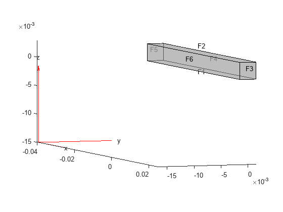
figure
pdegplot(gm,EdgeLabels="on",FaceAlpha=0.5)
view([71 4])
Add a vertex at the center of face 3.
centerVertex = addVertex(gm,Coordinates=[0.025 0 0.0015]);
Create an femodel object for transient structural analysis and include the geometry in the model.
model = femodel(AnalysisType="structuralTransient", ...
                 Geometry=gm);
Specify Young's modulus, Poisson's ratio, and the mass density of the material.
model.MaterialProperties = ...
    materialProperties(YoungsModulus=210E9, ...
                       PoissonsRatio=0.3, ...
                       MassDensity=7800);
Fix one end of the beam.
model.EdgeBC([2 8 11 12]) = edgeBC(Constraint="fixed");Generate a mesh. The mesh contains 590 elements and 1263 nodes. Each node has three translational DoFs. The total number of DoFs in this case is 3789.
model = generateMesh(model);
model.Geometry.Mesh
ans =
  FEMesh with properties:

             Nodes: [3×1277 double]
          Elements: [10×602 double]
    MaxElementSize: 0.0020
    MinElementSize: 0.0010
     MeshGradation: 1.5000
    GeometricOrder: 'quadratic'
Apply a sinusoidal concentrated force with the frequency 6000 and the amplitude 10 in the z-direction on the new vertex by using the helper function sinusoidalLoad.
Force = [0 0 10];
Frequency = 6000;
Phase = 0;
forcePulse = @(location,state) ...
    sinusoidalLoad(Force,location,state,Frequency,Phase);
model.VertexLoad(centerVertex) = vertexLoad(Force=forcePulse);
Specify zero initial conditions.
model.CellIC = cellIC(Velocity=[0 0 0],Displacement=[0 0 0]);
To estimate the computational effort required to solve the full model, find the sizes of the stiffness and mass matrices for this problem by assembling these matrices for the final time step.
tlist = 0:0.00005:3E-3;
state.time = tlist(end);
FEM = assembleFEMatrices(model,"KM",state)
FEM = struct with fields:
K: [3831×3831 double]
M: [3831×3831 double]
Reduce Model
Specify the fixed and loaded boundaries as structural superelement interfaces by creating a romInterface object for each superelement interface. The reduced-order model technique retains the DoFs on the superelement interfaces while condensing all other DoFs to a set of modal DoFs. For better performance, use the set of edges bounding face 5 instead of using the entire face.
romObj1 = romInterface(Edge=[2 8 11 12]);
romObj2 = romInterface(Vertex=centerVertex);
Assign a vector of interface objects to the ROMInterfaces property of the model.
model.ROMInterfaces = [romObj1,romObj2];
Reduce the structure, retaining all fixed interface modes up to 5e5. The reduced model has 51 retained DoFs, and the stiffness and mass matrices are 65-by-65.
rom = reduce(model,FrequencyRange=[-0.1,5e5])
rom =
  ReducedStructuralModel with properties:

                     K: [65×65 double]
                     M: [65×65 double]
              NumModes: 14
           RetainedDoF: [51×1 double]
    ReferenceLocations: []
                  Mesh: [1×1 FEMesh]
Simulate Transient Dynamics Using ROM
Next, use the reduced-order model to simulate the transient dynamics. Use the ode15s function directly to integrate the reduced system of ordinary differential equations. Take the loaded and modal DoFs for time-integration, and leave the fixed DoFs aside because the solution remains zero for those DoFs.
Working with the reduced model requires indexing into the reduced system matrices rom.K and rom.M. The arrangement of DoFs in reduced system is such that the physical DoFs corresponding to retained interfaces appear first followed by the generalized model DoFs. DoFs in a structural problem correspond to translational displacements. If the number of mesh points in a model is Nn, then the software assigns the IDs to the DoFs as follows: the first 1 to Nn are x-displacements, Nn+1 to 2*Nn are y-displacements, and 2Nn+1 to 3*Nn are z-displacements. Only the subset of these 3*Nn DoFs corresponding to ROMInterfaces is retained in the reduced model. The reduced model object rom contains these IDs for the retained DoFs in rom.RetainedDoF.
Create a function that returns DoF IDs given node IDs and the number of nodes.
getDoF = @(x,numNodes) [x(:); x(:) + numNodes; x(:) + 2*numNodes];
Find the node at the loaded vertex.
loadedNode = findNodes(rom.Mesh,"region",Vertex=centerVertex);Find the DoF of the loaded nodes using the helper function getDoF.
numNodes = size(rom.Mesh.Nodes,2);
loadDoFs = getDoF(loadedNode,numNodes);
Knowing the DoF IDs for the given node IDs, use rom.RetainedDoF and the intersect function to find the required indices corresponding to those DoF in the reduced matrices.
[~,loadNodeROMIds] = intersect(rom.RetainedDoF,loadDoFs);
In the reduced matrices rom.K and rom.M, generalized modal DoFs appear after the retained DoFs. Find the indices of modal DoFs in rom matrices.
modelDoFIDs = ((numel(rom.RetainedDoF) + 1):size(rom.K,1))';
Find the indices for the ODE DoFs in reduced matrices. Because fixed-end DoFs are not a part of the ODE system, these indices are as follows.
odeDoFs = [loadNodeROMIds;modelDoFIDs];
Find the relevant components of rom.K and rom.M for time integration.
Kconstrained = rom.K(odeDoFs,odeDoFs);
Mconstrained = rom.M(odeDoFs,odeDoFs);
numODE = numel(odeDoFs);
Now you have a second-order system of ODEs. To use ode15s, you must convert this system into a system of first-order ODEs by applying linearization. This type of a first-order system is twice the size of the second-order system.
Mode = [eye(numODE,numODE),   zeros(numODE,numODE); ...
        zeros(numODE,numODE), Mconstrained];
Kode = [zeros(numODE,numODE), -eye(numODE,numODE); ...
        Kconstrained,         zeros(numODE,numODE)];
Fode = zeros(2*numODE,1);
The specified concentrated force load in the full system is along the z-direction, which is the third DoF in the ODE system. Accounting for the linearization, obtain the first-order system to get the loaded ODE DoF.
loadODEDoF = numODE + 3;
Specify the mass matrix and the Jacobian for the ODE solver.
odeoptions = odeset;
odeoptions = odeset(odeoptions,"Jacobian",-Kode);
odeoptions = odeset(odeoptions,"Mass",Mode);
Specify zero initial conditions.
u0 = zeros(2*numODE,1);
Create the helper function specifying a sinusoidal concentrated force the vertex at the center of the front face (face 3). The force has the frequency 6000 and the amplitude 10 in the z-direction.
function f = CMSODEf(t,u,Kode,Fode,centerVertex)
Fode(centerVertex) = 10*sin(6000*t);
f = -Kode*u +Fode;
end
Solve the reduced system by using ode15s and the helper function. Use the tic command to start measuring the total time required to solve the reduced system and then reconstruct the full solution.
tic
sol = ode15s(@(t,y) CMSODEf(t,y,Kode,Fode,loadODEDoF), ...
                                 tlist,u0,odeoptions);
Compute the values of the ODE variable and the time derivatives.
[displ,vel] = deval(sol,tlist);
Reconstruct Solution for Full Model
Knowing the solution in terms of the interface DoFs and modal DoFs, you can reconstruct the solution for the full model. The reconstructSolution function requires the displacement, velocity, and acceleration at all DoFs in rom. Create the complete solution vector, including the zero values at the fixed DoFs.
u = zeros(size(rom.K,1),numel(tlist));
ut = zeros(size(rom.K,1),numel(tlist));
utt = zeros(size(rom.K,1),numel(tlist));
u(odeDoFs,:) = displ(1:numODE,:);
ut(odeDoFs,:) = vel(1:numODE,:);
utt(odeDoFs,:) = vel(numODE+1:2*numODE,:);
Create a transient results object using this solution. Use the toc command to report the elapsed time.
RTrom = reconstructSolution(rom,u,ut,utt,tlist);
toc
Elapsed time is 0.947855 seconds.
For comparison, solve the problem without using ROM and measure the time required to find the solution.
tic
result = solve(model,tlist);
toc
Elapsed time is 17.783697 seconds.
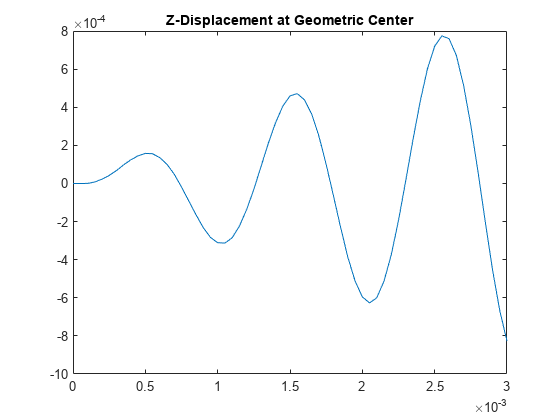
For both the direct and reconstructed solution, interpolate the displacement at the geometric center of the beam.
coordCenter = [0;0;0];
iDispRT = interpolateDisplacement(result,coordCenter);
iDispRTrom = interpolateDisplacement(RTrom,coordCenter);
Plot the interpolated displacement values. Overlapping plots prove that the reconstructed solution is very close to the direct solution. For better visibility, plot one of the solutions using the scatter function.
figure
plot(tlist,iDispRTrom.uz)
hold on
scatter(tlist,iDispRT.uz)
title("Z-Displacement at Geometric Center")
hold off
Sinusoidal Load Function
Define a sinusoidal load function, sinusoidalLoad, to model a harmonic load. This function accepts the load magnitude (amplitude), location and state structure arrays, frequency, and phase. Because the function depends on time, it must return a matrix of NaN of the correct size when state.time is NaN. Solvers check whether a problem is nonlinear or time-dependent by passing NaN state values and looking for returned NaN values.
function Tn = sinusoidalLoad(load,location,state,Frequency,Phase)
if isnan(state.time)
    normal = [location.nx location.ny];
    if isfield(location,"nz")
        normal = [normal location.nz];
    end
    Tn = NaN*normal;
    return
end
if isa(load,"function_handle")
    load = load(location,state);
else
    load = load(:);
end
% Transient model excited with harmonic load
Tn = load.*sin(Frequency.*state.time + Phase);
end
Reconstruct the solution for a full thermal transient analysis from the reduced-order model.
Create an femodel object for transient thermal analysis, and include a unit square geometry in the model.
model = femodel(AnalysisType="thermalTransient", ...
                Geometry=@squareg);
Plot the geometry, displaying edge labels.
pdegplot(model,EdgeLabels="on")
xlim([-1.1 1.1])
ylim([-1.1 1.1])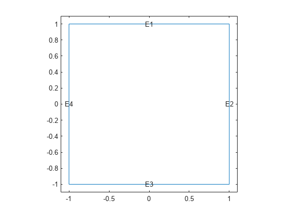
Specify the thermal conductivity, mass density, and specific heat of the material.
model.MaterialProperties = ...
    materialProperties(ThermalConductivity=400, ...
                       MassDensity=1300, ...
                       SpecificHeat=600);
Set the temperature on the right edge to 100.
model.EdgeBC(2) = edgeBC(Temperature=100);
Set an initial value of 50 for the temperature.
model.FaceIC = faceIC(Temperature=50);
Generate a mesh.
model = generateMesh(model);
Solve the model for three different values of heat source, and collect snapshots.
tlist = 0:10:600;
snapShotIDs = [1:10 59 60 61];
Tmatrix = [];

heatVariation = [10000 15000 20000];
for q = heatVariation
    model.FaceLoad = faceLoad(Heat=q);
    results = solve(model,tlist);
    Tmatrix = [Tmatrix,results.Temperature(:,snapShotIDs)];
end
Switch the thermal model analysis type to modal.
model.AnalysisType = "thermalModal";Compute the POD modes.
RModal = solve(model,Snapshots=Tmatrix);
Reduce the thermal model.
Rtherm = reduce(model,ModalResults=RModal)
Rtherm =
  ReducedThermalModel with properties:

                    K: [6×6 double]
                    M: [6×6 double]
                    F: [6×1 double]
    InitialConditions: [6×1 double]
                 Mesh: [1×1 FEMesh]
           ModeShapes: [1529×5 double]
     SnapshotsAverage: [1529×1 double]
Next, use the reduced-order model to simulate the transient dynamics. Use the ode15s function directly to integrate the reduced system ODE. Specify the mass matrix and the Jacobian for the ODE solver.
odeoptions = odeset;
odeoptions = odeset(odeoptions,Mass=Rtherm.M);
odeoptions = odeset(odeoptions,JConstant="on");
f = @(t,u) -Rtherm.K*u + Rtherm.F;
df = -Rtherm.K;
odeoptions = odeset(odeoptions,Jacobian=df);
Solve the reduced system by using ode15s.
sol = ode15s(f,tlist,Rtherm.InitialConditions,odeoptions);
Compute the values of the ODE variable.
u = deval(sol,tlist);
Reconstruct the solution for the full model.
R = reconstructSolution(Rtherm,u,tlist);
Plot the temperature distribution at the last time step.
pdeplot(R.Mesh,XYData=R.Temperature(:,end))
axis equal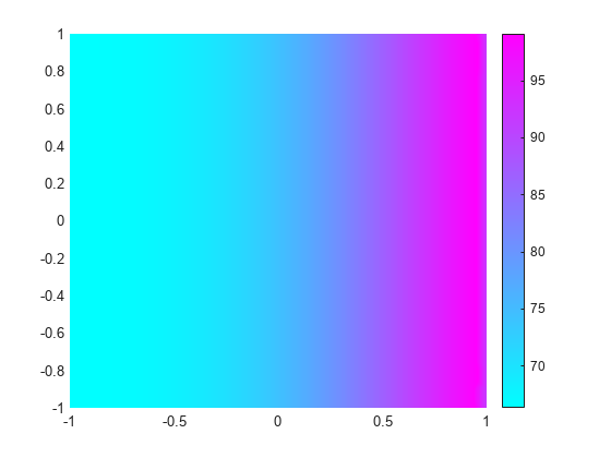
Input Arguments
Output Arguments
Version History
Introduced in R2019bSee Also
ReducedStructuralModel | ReducedThermalModel | ModalThermalResults | reduce | solve