uitimescope

Display time-domain signals in app

Since R2024a

Syntax

s = uitimescope

s = uitimescope(parent)

s = uitimescope(___,Name=Value)

Description

s = uitimescope creates a time scope UI component in a new figure and returns the TimeScope object. MATLAB^® calls the uifigure function to create the figure.

s = uitimescope(parent) creates a time scope UI component in the specified parent container. The parent can be a figure created using the uifigure function or one of its child containers.

s = uitimescope(___,Name=Value) specifies TimeScope properties using one or more name-value arguments. Use this option with any of the input argument combinations in the previous syntaxes. For example, uitimescope(Title="My Plot") specifies the time scope title. For a list of properties, see TimeScope Properties.

Examples

Create Time Scope

Create a time scope component in a UI figure.

fig = uifigure;
s = uitimescope(fig);

Set and Access Time Scope Properties

Create a time scope component in a UI figure. Specify the scope title.

fig = uifigure;
s = uitimescope(fig,Title="My Data");

Query the length of the x-axis range using the XTimeSpan property.

s.XTimeSpan

ans = 10

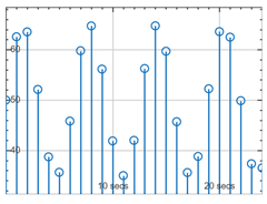
Update the x-axis time span to show 20 seconds of data.

s.XTimeSpan = 20;

Plot Signal Data on Time Scope

Visualize signal data in an app while a simulation runs by connecting a logged signal in a Simulink model to a time scope in an app.

First, create a time scope component in a UI figure.

fig = uifigure;
scope = uitimescope(fig);

Create a Simulation object that represents a simulation of the bouncingBall model and load the model.

s = simulation('bouncingBall',LoadModel=true);

Connect a logged signal in the model to the time scope component by creating a binding. Specify the binding source by using the collection of signals logged in the Simulation object along with the block path and port index of the specific signal to visualize. Specify the binding destination as the TimeScope object.

sig = s.LoggedSignals;
tindoors = s.ModelName + "/Second-Order  Integrator:1";
bind(sig,tindoors,scope);

Start the simulation. The time scope displays the signal data as the simulation runs.

start(s)

Input Arguments

parent — Parent container

Figure object (default) | Tab object | Panel object | ButtonGroup object | GridLayout object

Parent container, specified as a Figure object created using the uifigure or one of its child containers: a Tab, Panel, ButtonGroup, or GridLayout object. If you do not specify a parent container, MATLAB calls the uifigure function to create a new Figure object that serves as the parent container.

Name-Value Arguments

Specify optional pairs of arguments as Name1=Value1,...,NameN=ValueN, where Name is the argument name and Value is the corresponding value. Name-value arguments must appear after other arguments, but the order of the pairs does not matter.

Example: uitimescope(Title="My Plot")

Note

The properties listed here are a subset of the available properties. For the full list, see TimeScope Properties.

XTimeSpan — Length of x-axis range

10 (default) | positive value

Length of the x-axis range, in seconds, specified as a positive value. As new data displays in the time scope, the limits of the x-axis change to reflect the data. The value of XTimeSpan specifies how much data the time scope displays at any time.

Data Types: single | double | int8 | int16 | int32 | int64 | uint8 | uint16 | uint32 | uint64

YLimits — Minimum and maximum y-axis limits

[-10 10] (default) | two-element vector of the form [min max]

Minimum and maximum y-axis limits, specified as a two-element vector of the form [min max], where max is greater than min.

Data Types: single | double | int8 | int16 | int32 | int64 | uint8 | uint16 | uint32 | uint64

PlotType — Type of plot

'line' (default) | 'stairs' | 'stem'

Type of plot, specified as 'line', 'stairs', or 'stem'.

This table describes each of the plot types and when to use each type.

Value	Use	Appearance
'line'	Visualize continuous signals.
'stairs'	Visualize discrete signals.
'stem'	Visualize frequency of signal values.

Position — Size and location

[10 10 400 250] (default) | four-element vector of the form [left bottom width height]

Size and location, specified as a four-element vector of the form [left bottom width height]. This table describes each element of the vector.

Element	Description
left	Distance from the inner left edge of the parent container to the outer left edge of the scope
bottom	Distance from the inner bottom edge of the parent container to the outer bottom edge of the scope
width	Distance between the right and left outer edges of the scope
height	Distance between the top and bottom outer edges of the scope

All measurements are in pixel units.

Version History

Introduced in R2024a