Main Content

canoncorr

Canonical correlation

Description

[A,B] = canoncorr(X,Y) computes the sample canonical coefficients for the data matrices X and Y.

[A,B,r] = canoncorr(X,Y) also returns r, a vector of the sample canonical correlations.

example

[A,B,r,U,V] = canoncorr(X,Y) also returns U and V, matrices of the canonical scores for X and Y, respectively.

[A,B,r,U,V,stats] = canoncorr(X,Y) also returns stats, a structure containing information related to testing the sequence of hypotheses that the remaining correlations are all zero.

Examples

collapse all

Perform canonical correlation analysis for a sample data set.

The data set carbig contains measurements for 406 cars from the years 1970 to 1982.

Load the sample data.

load carbig;
data = [Displacement Horsepower Weight Acceleration MPG];

Define X as the matrix of displacement, horsepower, and weight observations, and Y as the matrix of acceleration and MPG observations. Omit rows with insufficient data.

nans = sum(isnan(data),2) > 0;
X = data(~nans,1:3);
Y = data(~nans,4:5);

Compute the sample canonical correlation.

[A,B,r,U,V] = canoncorr(X,Y);

View the output of A to determine the linear combinations of displacement, horsepower, and weight that make up the canonical variables of X.

A
A = 3×2

    0.0025    0.0048
    0.0202    0.0409
   -0.0000   -0.0027

A(3,1) is displayed as —0.000 because it is very small. Display A(3,1) separately.

A(3,1)
ans = -2.4737e-05

The first canonical variable of X is u1 = 0.0025*Disp + 0.0202*HP — 0.000025*Wgt.

The second canonical variable of X is u2 = 0.0048*Disp + 0.0409*HP — 0.0027*Wgt.

View the output of B to determine the linear combinations of acceleration and MPG that make up the canonical variables of Y.

B
B = 2×2

   -0.1666   -0.3637
   -0.0916    0.1078

The first canonical variable of Y is v1 = 0.1666*Accel — 0.0916*MPG.

The second canonical variable of Y is v2 = —0.3637*Accel + 0.1078*MPG.

Plot the scores of the canonical variables of X and Y against each other.

t = tiledlayout(2,2);
title(t,'Canonical Scores of X vs Canonical Scores of Y')
xlabel(t,'Canonical Variables of X')
ylabel(t,'Canonical Variables of Y')
t.TileSpacing = 'compact';

nexttile
plot(U(:,1),V(:,1),'.')
xlabel('u1')
ylabel('v1')

nexttile
plot(U(:,2),V(:,1),'.')
xlabel('u2')
ylabel('v1')

nexttile
plot(U(:,1),V(:,2),'.')
xlabel('u1')
ylabel('v2')

nexttile
plot(U(:,2),V(:,2),'.')
xlabel('u2')
ylabel('v2')
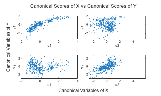
The pairs of canonical variables {ui,vi} are ordered from the strongest to weakest correlation, with all other pairs independent.

Return the correlation coefficient of the variables u1 and v1.

r(1)
ans = 0.8782

Input Arguments

collapse all

Input matrix, specified as an n-by-d1 matrix. The rows of X correspond to observations, and the columns correspond to variables.

Data Types: single | double

Input matrix, specified as an n-by-d2 matrix where X is an n-by-d1 matrix. The rows of Y correspond to observations, and the columns correspond to variables.

Data Types: single | double

Output Arguments

collapse all

Sample canonical coefficients for the variables in X, returned as a d1-by-d matrix, where d = min(rank(X),rank(Y)).

The jth column of A contains the linear combination of variables that makes up the jth canonical variable for X.

If X is less than full rank, canoncorr gives a warning and returns zeros in the rows of A corresponding to dependent columns of X.

Sample canonical coefficients for the variables in Y, returned as a d2-by-d matrix, where d = min(rank(X),rank(Y)).

The jth column of B contains the linear combination of variables that makes up the jth canonical variable for Y.

If Y is less than full rank, canoncorr gives a warning and returns zeros in the rows of B corresponding to dependent columns of Y.

Sample canonical correlations, returned as a 1-by-d vector, where d = min(rank(X),rank(Y)).

The jth element of r is the correlation between the jth columns of U and V.

Canonical scores for the variables in X, returned as an n-by-d matrix, where X is an n-by-d1 matrix and d = min(rank(X),rank(Y)).

Canonical scores for the variables in Y, returned as an n-by-d matrix, where Y is an n-by-d2 matrix and d = min(rank(X),rank(Y)).

Hypothesis test information, returned as a structure. This information relates to the sequence of d null hypotheses H0(k) that the (k+1)st through dth correlations are all zero for k=1,…,d-1, and d = min(rank(X),rank(Y)).

The fields of stats are 1-by-d vectors with elements corresponding to the values of k.

FieldDescription
Wilks

Wilks' lambda (likelihood ratio) statistic

df1

Degrees of freedom for the chi-squared statistic, and the numerator degrees of freedom for the F statistic

df2

Denominator degrees of freedom for the F statistic

F

Rao's approximate F statistic for H0(k)

pF

Right-tail significance level for F

chisq

Bartlett's approximate chi-squared statistic for H0(k) with Lawley's modification

pChisq

Right-tail significance level for chisq

stats has two other fields (dfe and p), which are equal to df1 and pChisq, respectively, and exist for historical reasons.

Data Types: struct

More About

collapse all

Canonical Correlation Analysis

The canonical scores of the data matrices X and Y are defined as

Ui=XaiVi=Ybi

where ai and bi maximize the Pearson correlation coefficient ρ(Ui,Vi) subject to being uncorrelated to all previous canonical scores and scaled so that Ui and Vi have zero mean and unit variance.

The canonical coefficients of X and Y are the matrices A and B with columns ai and bi, respectively.

The canonical variables of X and Y are the linear combinations of the columns of X and Y given by the canonical coefficients in A and B respectively.

The canonical correlations are the values ρ(Ui,Vi) measuring the correlation of each pair of canonical variables of X and Y.

Algorithms

canoncorr computes A, B, and r using qr and svd. canoncorr computes U and V as U = (X—mean(X))*A and V = (Y—mean(Y))*B.

References

[1] Krzanowski, W. J. Principles of Multivariate Analysis: A User's Perspective. New York: Oxford University Press, 1988.

[2] Seber, G. A. F. Multivariate Observations. Hoboken, NJ: John Wiley & Sons, Inc., 1984.

Version History

Introduced before R2006a

See Also

|