plot

Plot bar graph of fairness metric

Since R2022b

Syntax

plot(metricsResults,metric)

plot(metricsResults,metric,Name=Value)

plot(ax,___)

b = plot(___)

Description

plot(metricsResults,metric) creates a bar graph of the specified metric (metric), stored in either the BiasMetrics or GroupMetrics property of the fairnessMetrics object (metricsResults). By default, the function creates a graph for the first attribute stored in the SensitiveAttributeNames property of metricsResults.

If you specified predicted class labels for multiple models when you created metricsResults, then the graph includes bars of different colors, where the color indicates the model.

plot(metricsResults,metric,Name=Value) specifies additional options using one or more name-value arguments. For example, you can specify the sensitive attribute to plot by using the SensitiveAttributeName name-value argument.

plot(ax,___) displays the plot in the target axes ax. Specify the axes as the first argument in any of the previous syntaxes. (since R2023b)

b = plot(___) returns a Bar object or an array of Bar objects. Use b to query or modify Bar Properties after displaying the bar graph.

Examples

Specify Fairness Metric to Plot

Compute fairness metrics for true labels with respect to sensitive attributes by creating a fairnessMetrics object. Then, plot a bar graph of a specified metric by using the plot function.

Read the sample file CreditRating_Historical.dat into a table. The predictor data consists of financial ratios and industry sector information for a list of corporate customers. The response variable consists of credit ratings assigned by a rating agency.

creditrating = readtable("CreditRating_Historical.dat");

Because each value in the ID variable is a unique customer ID—that is, length(unique(creditrating.ID)) is equal to the number of observations in creditrating—the ID variable is a poor predictor. Remove the ID variable from the table, and convert the Industry variable to a categorical variable.

creditrating.ID = [];
creditrating.Industry = categorical(creditrating.Industry);

In the Rating response variable, combine the AAA, AA, A, and BBB ratings into a category of "good" ratings, and the BB, B, and CCC ratings into a category of "poor" ratings.

Rating = categorical(creditrating.Rating);
Rating = mergecats(Rating,["AAA","AA","A","BBB"],"good");
Rating = mergecats(Rating,["BB","B","CCC"],"poor");
creditrating.Rating = Rating;

Compute fairness metrics with respect to the sensitive attribute Industry for the labels in the Rating variable.

metricsResults = fairnessMetrics(creditrating,"Rating", ...
    SensitiveAttributeNames="Industry");

fairnessMetrics computes metrics for all supported bias and group metrics. Display the names of the metrics stored in the BiasMetrics and GroupMetrics properties.

metricsResults.BiasMetrics.Properties.VariableNames(3:end)'

ans = 2×1 cell
    {'StatisticalParityDifference'}
    {'DisparateImpact'            }

metricsResults.GroupMetrics.Properties.VariableNames(3:end)'

ans = 2×1 cell
    {'GroupCount'    }
    {'GroupSizeRatio'}

Create a bar graph of the disparate impact values.

plot(metricsResults,"DisparateImpact")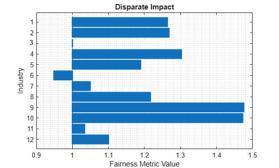

Specify Sensitive Attribute to Plot

Compute fairness metrics for predicted labels with respect to sensitive attributes by creating a fairnessMetrics object. Then, plot a bar graph of a specified metric and sensitive attribute by using the plot function.

Load the sample data census1994, which contains the training data adultdata and the test data adulttest. The data sets consist of demographic information from the US Census Bureau that can be used to predict whether an individual makes over $50,000 per year. Preview the first few rows of the training data set.

load census1994
head(adultdata)

    age       workClass          fnlwgt      education    education_num       marital_status           occupation        relationship     race      sex      capital_gain    capital_loss    hours_per_week    native_country    salary
    ___    ________________    __________    _________    _____________    _____________________    _________________    _____________    _____    ______    ____________    ____________    ______________    ______________    ______

    39     State-gov                77516    Bachelors         13          Never-married            Adm-clerical         Not-in-family    White    Male          2174             0                40          United-States     <=50K 
    50     Self-emp-not-inc         83311    Bachelors         13          Married-civ-spouse       Exec-managerial      Husband          White    Male             0             0                13          United-States     <=50K 
    38     Private             2.1565e+05    HS-grad            9          Divorced                 Handlers-cleaners    Not-in-family    White    Male             0             0                40          United-States     <=50K 
    53     Private             2.3472e+05    11th               7          Married-civ-spouse       Handlers-cleaners    Husband          Black    Male             0             0                40          United-States     <=50K 
    28     Private             3.3841e+05    Bachelors         13          Married-civ-spouse       Prof-specialty       Wife             Black    Female           0             0                40          Cuba              <=50K 
    37     Private             2.8458e+05    Masters           14          Married-civ-spouse       Exec-managerial      Wife             White    Female           0             0                40          United-States     <=50K 
    49     Private             1.6019e+05    9th                5          Married-spouse-absent    Other-service        Not-in-family    Black    Female           0             0                16          Jamaica           <=50K 
    52     Self-emp-not-inc    2.0964e+05    HS-grad            9          Married-civ-spouse       Exec-managerial      Husband          White    Male             0             0                45          United-States     >50K  

Each row contains the demographic information for one adult. The information includes sensitive attributes, such as age, marital_status, relationship, race, and sex. The third column flnwgt contains observation weights, and the last column salary shows whether a person has a salary less than or equal to $50,000 per year (<=50K) or greater than $50,000 per year (>50K).

Train a classification tree using the training data set adultdata. Specify the response variable, predictor variables, and observation weights by using the variable names in the adultdata table.

predictorNames = ["capital_gain","capital_loss","education", ...
    "education_num","hours_per_week","occupation","workClass"];
Mdl = fitctree(adultdata,"salary", ...
    PredictorNames=predictorNames,Weights="fnlwgt");

Predict the test sample labels by using the trained tree Mdl.

adulttest.predictions = predict(Mdl,adulttest);

This example evaluates the fairness of the predicted labels with respect to age and marital status. Group the age variable into four bins.

ageGroups = ["Age<30","30<=Age<45","45<=Age<60","Age>=60"];
adulttest.age_group = discretize(adulttest.age, ...
    [min(adulttest.age) 30 45 60 max(adulttest.age)], ...
    categorical=ageGroups);

Compute fairness metrics for the predictions with respect to the age_group and marital_status variables by using fairnessMetrics.

metricsResults = fairnessMetrics(adulttest,"salary", ...
    SensitiveAttributeNames=["age_group","marital_status"], ...
    Predictions="predictions",Weights="fnlwgt")

metricsResults = 
  fairnessMetrics with properties:

    SensitiveAttributeNames: {'age_group'  'marital_status'}
             ReferenceGroup: {'30<=Age<45'  'Married-civ-spouse'}
               ResponseName: 'salary'
              PositiveClass: >50K
                BiasMetrics: [11×7 table]
               GroupMetrics: [11×20 table]
                 ModelNames: 'predictions'


  Properties, Methods

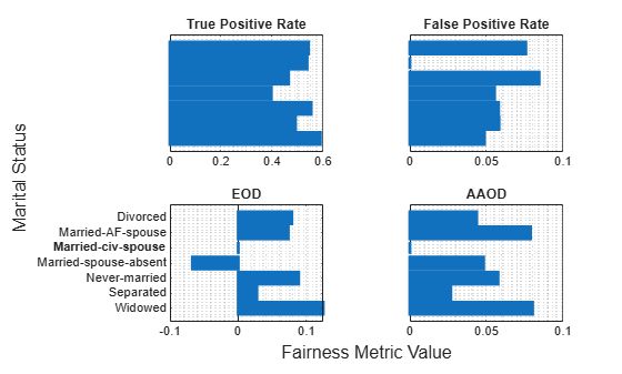
Create bar graphs of the true positive rate (TPR), false positive rate (FPR), equal opportunity difference (EOD), and average absolute odds difference (AAOD) values for the sensitive attribute marital_status. The default value of the SensitiveAttributeName argument is the first element in the SensitiveAttributeNames property of the fairnessMetrics object. In this case, the first element is age_group. Specify SensitiveAttributeName as marital_status.

t = tiledlayout(2,2);
nexttile
plot(metricsResults,"tpr",SensitiveAttributeName="marital_status")
xlabel("")
ylabel("")
nexttile
plot(metricsResults,"fpr",SensitiveAttributeName="marital_status")
yticklabels("")
xlabel("")
ylabel("")
nexttile
plot(metricsResults,"eod",SensitiveAttributeName="marital_status")
xlabel("")
ylabel("")
title("EOD")
nexttile
plot(metricsResults,"aaod",SensitiveAttributeName="marital_status")
yticklabels("")
xlabel("")
ylabel("")
title("AAOD")
xlabel(t,"Fairness Metric Value")
ylabel(t,"Marital Status")

Compare Model Predictions Using Fairness Metrics

Train two classification models, and compare the model predictions by using fairness metrics.

Read the sample file CreditRating_Historical.dat into a table. The predictor data consists of financial ratios and industry sector information for a list of corporate customers. The response variable consists of credit ratings assigned by a rating agency.

creditrating = readtable("CreditRating_Historical.dat");

Because each value in the ID variable is a unique customer ID—that is, length(unique(creditrating.ID)) is equal to the number of observations in creditrating—the ID variable is a poor predictor. Remove the ID variable from the table, and convert the Industry variable to a categorical variable.

creditrating.ID = [];
creditrating.Industry = categorical(creditrating.Industry);

In the Rating response variable, combine the AAA, AA, A, and BBB ratings into a category of "good" ratings, and the BB, B, and CCC ratings into a category of "poor" ratings.

Rating = categorical(creditrating.Rating);
Rating = mergecats(Rating,["AAA","AA","A","BBB"],"good");
Rating = mergecats(Rating,["BB","B","CCC"],"poor");
creditrating.Rating = Rating;

Train a support vector machine (SVM) model on the creditrating data. For better results, standardize the predictors before fitting the model. Use the trained model to predict labels and compute the misclassification rate for the training data set.

predictorNames = ["WC_TA","RE_TA","EBIT_TA","MVE_BVTD","S_TA"];
SVMMdl = fitcsvm(creditrating,"Rating", ...
    PredictorNames=predictorNames,Standardize=true);
SVMPredictions = resubPredict(SVMMdl);
resubLoss(SVMMdl)

ans = 
0.0872

Train a generalized additive model (GAM).

GAMMdl = fitcgam(creditrating,"Rating", ...
    PredictorNames=predictorNames);
GAMPredictions = resubPredict(GAMMdl);
resubLoss(GAMMdl)

ans = 
0.0542

GAMMdl achieves better accuracy on the training data set.

Compute fairness metrics with respect to the sensitive attribute Industry by using the model predictions for both models.

predictions = [SVMPredictions,GAMPredictions];
metricsResults = fairnessMetrics(creditrating,"Rating", ...
    SensitiveAttributeNames="Industry",Predictions=predictions, ...
    ModelNames=["SVM","GAM"]);

Display the bias metrics by using the report function.

report(metricsResults)

ans=48×5 table
              Metrics              SensitiveAttributeNames    Groups       SVM          GAM    
    ___________________________    _______________________    ______    _________    __________

    StatisticalParityDifference           Industry              1       -0.028441     0.0058208
    StatisticalParityDifference           Industry              2        -0.04014     0.0063339
    StatisticalParityDifference           Industry              3               0             0
    StatisticalParityDifference           Industry              4        -0.04905    -0.0043007
    StatisticalParityDifference           Industry              5       -0.015615     0.0041607
    StatisticalParityDifference           Industry              6        -0.03818     -0.024515
    StatisticalParityDifference           Industry              7        -0.01514      0.007326
    StatisticalParityDifference           Industry              8       0.0078632      0.036581
    StatisticalParityDifference           Industry              9       -0.013863      0.042266
    StatisticalParityDifference           Industry              10      0.0090218      0.050095
    StatisticalParityDifference           Industry              11      -0.004188      0.001453
    StatisticalParityDifference           Industry              12      -0.041572     -0.028589
    DisparateImpact                       Industry              1         0.92261         1.017
    DisparateImpact                       Industry              2         0.89078        1.0185
    DisparateImpact                       Industry              3               1             1
    DisparateImpact                       Industry              4         0.86654       0.98742
      ⋮

Among the bias metrics, compare the equal opportunity difference (EOD) values. Create a bar graph of the EOD values by using the plot function.

b = plot(metricsResults,"eod");
b(1).FaceAlpha = 0.2;
b(2).FaceAlpha = 0.2;
legend(Location="southwest")

To better understand the distributions of EOD values, plot the values using box plots.

boxchart(metricsResults.BiasMetrics.EqualOpportunityDifference, ...
    GroupByColor=metricsResults.BiasMetrics.ModelNames)
ax = gca;
ax.XTick = [];
ylabel("Equal Opportunity Difference")
legend

The EOD values for GAM are closer to 0 compared to the values for SVM.

Input Arguments

metricsResults — Fairness metrics results

fairnessMetrics object

Fairness metrics results, specified as a fairnessMetrics object.

metric — Fairness metric to plot

string scalar | character vector

Fairness metric to plot, specified as a bias or group metric stored in either the BiasMetrics or GroupMetrics property of the fairnessMetrics object (metricsResults). The properties in metricsResults use full names for the table variable names. However, you can use either the full name or short name given in the following tables to specify the metric argument.

• Bias metrics

  Metric Name	Description	Evaluation Type
  "StatisticalParityDifference" or "spd"	Statistical parity difference (SPD)	Data-level or model-level evaluation
  "DisparateImpact" or "di"	Disparate impact (DI)	Data-level or model-level evaluation
  "EqualOpportunityDifference" or "eod"	Equal opportunity difference (EOD)	Model-level evaluation
  "AverageAbsoluteOddsDifference" or "aaod"	Average absolute odds difference (AAOD)	Model-level evaluation

  For definitions of the bias metrics, see Bias Metrics.

• Group metrics

  Metric Name	Description	Evaluation Type
  "GroupCount"	Group count, or number of samples in the group	Data-level or model-level evaluation
  "GroupSizeRatio"	Group count divided by the total number of samples	Data-level or model-level evaluation
  "TruePositives" or "tp"	Number of true positives (TP)	Model-level evaluation
  "TrueNegatives" or "tn"	Number of true negatives (TN)	Model-level evaluation
  "FalsePositives" or "fp"	Number of false positives (FP)	Model-level evaluation
  "FalseNegatives" or "fn"	Number of false negatives (FN)	Model-level evaluation
  "TruePositiveRate" or "tpr"	True positive rate (TPR), also known as recall or sensitivity, TP/(TP+FN)	Model-level evaluation
  "TrueNegativeRate", "tnr", or "spec"	True negative rate (TNR), or specificity, TN/(TN+FP)	Model-level evaluation
  "FalsePositiveRate" or "fpr"	False positive rate (FPR), also known as fallout or 1-specificity, FP/(TN+FP)	Model-level evaluation
  "FalseNegativeRate", "fnr", or "miss"	False negative rate (FNR), or miss rate, FN/(TP+FN)	Model-level evaluation
  "FalseDiscoveryRate" or "fdr"	False discovery rate (FDR), FP/(TP+FP)	Model-level evaluation
  "FalseOmissionRate" or "for"	False omission rate (FOR), FN/(TN+FN)	Model-level evaluation
  "PositivePredictiveValue", "ppv", or "prec"	Positive predictive value (PPV), or precision, TP/(TP+FP)	Model-level evaluation
  "NegativePredictiveValue" or "npv"	Negative predictive value (NPV), TN/(TN+FN)	Model-level evaluation
  "RateOfPositivePredictions" or "rpp"	Rate of positive predictions (RPP), (TP+FP)/(TP+FN+FP+TN)	Model-level evaluation
  "RateOfNegativePredictions" or "rnp"	Rate of negative predictions (RNP), (TN+FN)/(TP+FN+FP+TN)	Model-level evaluation
  "Accuracy" or "accu"	Accuracy, (TP+TN)/(TP+FN+FP+TN)	Model-level evaluation

A fairnessMetrics object stores bias and group metrics in the BiasMetrics and GroupMetrics properties, respectively. The supported metrics depend on whether you specify predicted labels by using the Predictions argument when you create the fairnessMetrics object.

• Data-level evaluation — If you specify true labels and do not specify predicted labels, the BiasMetrics property contains only StatisticalParityDifference and DisparateImpact, and the GroupMetrics property contains only GroupCount and GroupSizeRatio.

• Model-level evaluation — If you specify both true labels and predicted labels, BiasMetrics and GroupMetrics contain all metrics listed in the tables.

Data Types: char | string

ax — Axes for plot

Axes object

Since R2023b

Axes for the plot, specified as an Axes object. If you do not specify ax, then plot creates the plot using the current axes. For more information on creating an Axes object, see axes.

Name-Value Arguments

Specify optional pairs of arguments as Name1=Value1,...,NameN=ValueN, where Name is the argument name and Value is the corresponding value. Name-value arguments must appear after other arguments, but the order of the pairs does not matter.

Example: SensitiveAttributeName="Age",ModelNames="Tree" specifies to plot fairness metric values for the Age sensitive attribute, computed using the Tree model predicted labels.

SensitiveAttributeName — Name of sensitive attribute to plot

metricsResults.SensitiveAttributeNames{1} (default) | character vector | string scalar

Name of the sensitive attribute to plot, specified as a character vector or string scalar. The sensitive attribute name must be a name in the SensitiveAttributeNames property of metricsResults.

Example: SensitiveAttributeName="race"

Data Types: char | string

ModelNames — Names of models to plot

"all" (default) | character vector | string array | cell array of character vectors

Since R2023a

Names of the models to plot, specified as "all", a character vector, a string array, or a cell array of character vectors. The ModelNames value must contain names in the ModelNames property of metricsResults. Using the "all" value is equivalent to specifying metricsResults.ModelNames.

Example: ModelNames="Tree"

Example: ModelNames=["SVM","Neural Network"]

Data Types: char | string | cell

More About

Bias Metrics

The fairnessMetrics object supports four bias metrics: statistical parity difference (SPD), disparate impact (DI), equal opportunity difference (EOD), and average absolute odds difference (AAOD). The object supports EOD and AAOD only for evaluating model predictions.

A fairnessMetrics object computes bias metrics for each group in each sensitive attribute with respect to the reference group of the attribute.

• Statistical parity (or demographic parity) difference (SPD)

  The SPD value of the ith sensitive attribute (S_i) for the group s_ij with respect to the reference group s_ir is defined by

  $${\text{SPD}}_{ij}=P\left(Y=+|S_i=s_{ij}\right)-P\left(Y=+|S_i=s_{ir}\right).$$

  The SPD value is the difference between the probability of being in the positive class when the sensitive attribute value is s_ij and the probability of being in the positive class when the sensitive attribute value is s_ir (reference group). This metric assumes that the two probabilities (statistical parities) are equal if the labels are unbiased with respect to the sensitive attribute.

  If you specify the Predictions argument, the software computes SPD for the probabilities of the model predictions $$\widehat{Y}$$ instead of the true labels Y.

• Disparate impact (DI)

  The DI value of the ith sensitive attribute (S_i) for the group s_ij with respect to the reference group s_ir is defined by

  $${\text{DI}}_{ij}=\frac{P\left(Y=+|S_i=s_{ij}\right)}{P\left(Y=+|S_i=s_{ir}\right)}.$$

  The DI value is the ratio of the probability of being in the positive class when the sensitive attribute value is s_ij to the probability of being in the positive class when the sensitive attribute value is s_ir (reference group). This metric assumes that the two probabilities are equal if the labels are unbiased with respect to the sensitive attribute. In general, a DI value less than 0.8 or greater than 1.25 indicates bias with respect to the reference group [2].

  If you specify the Predictions argument, the software computes DI for the probabilities of the model predictions $$\widehat{Y}$$ instead of the true labels Y.

• Equal opportunity difference (EOD)

  The EOD value of the ith sensitive attribute (S_i) for the group s_ij with respect to the reference group s_ir is defined by

  $$\begin{array}{c}{\text{EOD}}_{ij}=\text{TPR}\left(S_i=s_{ij}\right)-\text{TPR}\left(S_i=s_{ir}\right)\\ =P\left(\widehat{Y}=+|Y=+,S_i=s_{ij}\right)-P\left(\widehat{Y}=+|Y=+,S_i=s_{ir}\right).\end{array}$$

  The EOD value is the difference in the true positive rate (TPR) between the group s_ij and the reference group s_ir. This metric assumes that the two rates are equal if the predicted labels are unbiased with respect to the sensitive attribute.

• Average absolute odds difference (AAOD)

  The AAOD value of the ith sensitive attribute (S_i) for the group s_ij with respect to the reference group s_ir is defined by

  $${\text{AAOD}}_{ij}=\frac{1}{2}\left(\left|\text{FPR}\left(S_i=s_{ij}\right)-\text{FPR}\left(S_i=s_{ir}\right)\right|+\left|\text{TPR}\left(S_i=s_{ij}\right)-\text{TPR}\left(S_i=s_{ir}\right)\right|\right).$$

  The AAOD value represents the difference in the true positive rates (TPR) and false positive rates (FPR) between the group s_ij and the reference group s_ir. This metric assumes no difference in TPR and FPR if the predicted labels are unbiased with respect to the sensitive attribute.

References

[1] Mehrabi, Ninareh, et al. “A Survey on Bias and Fairness in Machine Learning.” ArXiv:1908.09635 [cs.LG], Sept. 2019. arXiv.org.

[2] Saleiro, Pedro, et al. “Aequitas: A Bias and Fairness Audit Toolkit.” ArXiv:1811.05577 [cs.LG], April 2019. arXiv.org.

Version History

Introduced in R2022b

R2023b: plot uses specified target axes

You can now specify target axes for the plot object function. Specify an Axes object as the first input argument of the function.

R2023a: Compare fairness metrics across models

You can compare fairness metrics across multiple binary classifiers by using the fairnessMetrics function. In the call to the function, use the predictions argument and specify the predicted class labels for each model. To specify the names of the models, you can use the ModelNames name-value argument. The model name information is stored in the BiasMetrics, GroupMetrics, and ModelNames properties of the fairnessMetrics object.

After you create a fairnessMetrics object, use the report or plot object function.

• The report object function returns a fairness metrics table, whose format depends on the value of the DisplayMetricsInRows name-value argument. (For more information, see metricsTbl.) You can specify a subset of models to include in the report table by using the ModelNames name-value argument.

• The plot object function returns a bar graph as an array of Bar objects. The bar colors indicate the models whose predicted labels are used to compute the specified metric. You can specify a subset of models to include in the plot by using the ModelNames name-value argument.

In previous releases, the b = plot(__) syntax always returned a single Bar object. plot displayed blue bars with black edges for the metric values and a solid line for the baseline value. Now, the color of each bar edge matches the color of its bar, and the plot includes a dashed line for the baseline value.