fairnessThresholder
Description
fairnessThresholder searches for an optimal score threshold
to maximize accuracy while satisfying fairness bounds. For observations in the critical region
below the optimal threshold, the function adjusts the labels so that the fairness constraints
hold for the reference and nonreference groups in the sensitive attribute. After you create a
fairnessThresholder object, you can use the predict and
loss object
functions on new data to predict fairness labels and calculate the classification loss,
respectively.
Creation
Syntax
Description
fairnessMdl = fairnessThresholder(Mdl,Tbl,AttributeName,ResponseVarName)Mdl while
satisfying fairness bounds. The function tries a vector of thresholds for classifying
observations in the validation data table Tbl with the class labels
in the ResponseVarName table variable. For observations in the
critical region below the optimal threshold, the function adjusts the labels so that the
fairness constraints hold for the reference and nonreference groups in the
AttributeName sensitive attribute. For more information, see Reject Option-Based Classification.
fairnessMdl = fairnessThresholder(___,Name=Value)BiasMetric name-value argument.
Input Arguments
Name-Value Arguments
Properties
Object Functions
Examples
Train a tree ensemble for binary classification, and compute the disparate impact for each group in the sensitive attribute. To reduce the disparate impact value of the nonreference group, adjust the score threshold for classifying observations.
Load the data census1994, which contains the data set adultdata and the test data set adulttest. The data sets consist of demographic information from the US Census Bureau that can be used to predict whether an individual makes over $50,000 per year. Preview the first few rows of adultdata.
load census1994
head(adultdata)
age workClass fnlwgt education education_num marital_status occupation relationship race sex capital_gain capital_loss hours_per_week native_country salary
___ ________________ __________ _________ _____________ _____________________ _________________ _____________ _____ ______ ____________ ____________ ______________ ______________ ______
39 State-gov 77516 Bachelors 13 Never-married Adm-clerical Not-in-family White Male 2174 0 40 United-States <=50K
50 Self-emp-not-inc 83311 Bachelors 13 Married-civ-spouse Exec-managerial Husband White Male 0 0 13 United-States <=50K
38 Private 2.1565e+05 HS-grad 9 Divorced Handlers-cleaners Not-in-family White Male 0 0 40 United-States <=50K
53 Private 2.3472e+05 11th 7 Married-civ-spouse Handlers-cleaners Husband Black Male 0 0 40 United-States <=50K
28 Private 3.3841e+05 Bachelors 13 Married-civ-spouse Prof-specialty Wife Black Female 0 0 40 Cuba <=50K
37 Private 2.8458e+05 Masters 14 Married-civ-spouse Exec-managerial Wife White Female 0 0 40 United-States <=50K
49 Private 1.6019e+05 9th 5 Married-spouse-absent Other-service Not-in-family Black Female 0 0 16 Jamaica <=50K
52 Self-emp-not-inc 2.0964e+05 HS-grad 9 Married-civ-spouse Exec-managerial Husband White Male 0 0 45 United-States >50K
Each row contains the demographic information for one adult. The information includes sensitive attributes, such as age, marital_status, relationship, race, and sex. The third column flnwgt contains observation weights, and the last column salary shows whether a person has a salary less than or equal to $50,000 per year (<=50K) or greater than $50,000 per year (>50K).
Remove observations with missing values.
adultdata = rmmissing(adultdata);
adulttest = rmmissing(adulttest);
Partition adultdata into training and validation sets. Use 60% of the observations for the training set trainingData and 40% of the observations for the validation set validationData.
rng("default") % For reproducibility
c = cvpartition(adultdata.salary,"Holdout",0.4);
trainingIdx = training(c);
validationIdx = test(c);
trainingData = adultdata(trainingIdx,:);
validationData = adultdata(validationIdx,:);
Train a boosted ensemble of trees using the training data set trainingData. Specify the response variable, predictor variables, and observation weights by using the variable names in the adultdata table. Use random undersampling boosting as the ensemble aggregation method.
predictors = ["capital_gain","capital_loss","education", ...
    "education_num","hours_per_week","occupation","workClass"];
Mdl = fitcensemble(trainingData,"salary", ...
    PredictorNames=predictors, ...
    Weights="fnlwgt",Method="RUSBoost");
Predict salary values for the observations in the test data set adulttest, and calculate the classification error.
labels = predict(Mdl,adulttest);
L = loss(Mdl,adulttest)
L =
0.2080
The model accurately predicts the salary categorization for approximately 80% of the test set observations.
Compute fairness metrics with respect to the sensitive attribute sex by using the test set model predictions. In particular, find the disparate impact for each group in sex. Use the report and plot object functions of fairnessMetrics to display the results.
metricsResults = fairnessMetrics(adulttest,"salary", ...
    SensitiveAttributeNames="sex",Predictions=labels, ...
    ModelNames="Ensemble",Weights="fnlwgt");
metricsResults.PositiveClass
ans = categorical
     >50K
metricsResults.ReferenceGroup
ans =
'Male'
report(metricsResults,BiasMetrics="DisparateImpact")ans=2×4 table
ModelNames SensitiveAttributeNames Groups DisparateImpact
__________ _______________________ ______ _______________
Ensemble sex Female 0.73792
Ensemble sex Male 1
plot(metricsResults,"DisparateImpact")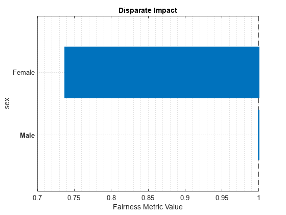
For the nonreference group (Female), the disparate impact value is the proportion of predictions in the group with a positive class value (>50K) divided by the proportion of predictions in the reference group (Male) with a positive class value. Ideally, disparate impact values are close to 1.
To try to improve the nonreference group disparate impact value, you can adjust model predictions by using the fairnessThresholder function. The function uses validation data to search for an optimal score threshold that maximizes accuracy while satisfying fairness bounds. For observations in the critical region below the optimal threshold, the function changes the labels so that the fairness constraints hold for the reference and nonreference groups. By default, the function tries to find a score threshold so that the disparate impact value for the nonreference group is in the range [0.8,1.25].
fairnessMdl = fairnessThresholder(Mdl,validationData,"sex","salary")
fairnessMdl =
  fairnessThresholder with properties:

               Learner: [1×1 classreg.learning.classif.CompactClassificationEnsemble]
    SensitiveAttribute: 'sex'
       ReferenceGroups: Male
          ResponseName: 'salary'
         PositiveClass: >50K
        ScoreThreshold: 1.6749
            BiasMetric: 'DisparateImpact'
       BiasMetricValue: 0.9702
       BiasMetricRange: [0.8000 1.2500]
        ValidationLoss: 0.2017
fairnessMdl is a fairnessThresholder model object. Note that the predict function of the ensemble model Mdl returns scores that are not posterior probabilities. Scores are in the range instead, and the maximum score for each observation is greater than 0. For observations whose maximum scores are less than the new score threshold (fairnessMdl.ScoreThreshold), the predict function of the fairnessMdl object adjusts the prediction. If the observation is in the nonreference group, the function predicts the observation into the positive class. If the observation is in the reference group, the function predicts the observation into the negative class. These adjustments do not always result in a change in the predicted label.
Adjust the test set predictions by using the new score threshold, and calculate the classification error.
fairnessLabels = predict(fairnessMdl,adulttest);
fairnessLoss = loss(fairnessMdl,adulttest)
fairnessLoss =
0.2064
The new classification error is similar to the original classification error.
Compare the disparate impact values across the two sets of test predictions: the original predictions computed using Mdl and the adjusted predictions computed using fairnessMdl.
newMetricsResults = fairnessMetrics(adulttest,"salary", ...
    SensitiveAttributeNames="sex",Predictions=[labels,fairnessLabels], ...
    ModelNames=["Original","Adjusted"],Weights="fnlwgt");
newMetricsResults.PositiveClass
ans = categorical
     >50K
newMetricsResults.ReferenceGroup
ans =
'Male'
report(newMetricsResults,BiasMetrics="DisparateImpact")ans=2×5 table
Metrics SensitiveAttributeNames Groups Original Adjusted
_______________ _______________________ ______ ________ ________
DisparateImpact sex Female 0.73792 1.0048
DisparateImpact sex Male 1 1
plot(newMetricsResults,"di")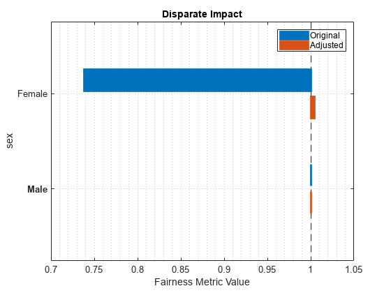
The disparate impact value for the nonreference group (Female) is closer to 1 when you use the adjusted predictions.
Train a support vector machine (SVM) model, and compute the statistical parity difference (SPD) for each group in the sensitive attribute. To reduce the SPD value of the nonreference group, adjust the score threshold for classifying observations.
Load the patients data set, which contains medical information for 100 patients. Convert the Gender and Smoker variables to categorical variables. Specify the descriptive category names Smoker and Nonsmoker rather than 1 and 0.
load patients
Gender = categorical(Gender);
Smoker = categorical(Smoker,logical([1 0]), ...
    ["Smoker","Nonsmoker"]);
Create a matrix containing the continuous predictors Diastolic and Systolic. Specify Gender as the sensitive attribute and Smoker as the response variable.
X = [Diastolic,Systolic];
attribute = Gender;
Y = Smoker;
Partition the data into training and validation sets. Use half of the observations for training and half of the observations for validation.
rng("default") % For reproducibility
cv = cvpartition(Y,"Holdout",0.5);

trainX = X(training(cv),:);
trainAttribute = attribute(training(cv));
trainY = Y(training(cv));

validationX = X(test(cv),:);
validationAttribute = attribute(test(cv));
validationY = Y(test(cv));
Train a support vector machine (SVM) binary classifier on the training data. Standardize the predictors before fitting the model. Use the trained model to predict labels and compute scores for the validation data set.
mdl = fitcsvm(trainX,trainY,Standardize=true);
[labels,scores] = predict(mdl,validationX);
For the validation data set, combine the sensitive attribute and response variable information into one grouping variable groupTest.
groupTest = validationAttribute.*validationY;
names = string(categories(groupTest))
names = 4×1 string
    "Female Smoker"
    "Female Nonsmoker"
    "Male Smoker"
    "Male Nonsmoker"
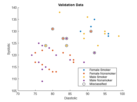
Find the validation observations that are misclassified by the SVM model.
wrongIdx = (validationY ~= labels);
wrongX = validationX(wrongIdx,:);
names(5) = "Misclassified";
Plot the validation data. The color of each point indicates the sensitive attribute group and class label for that observation. Circled points indicate misclassified observations.
figure
hold on
gscatter(validationX(:,1),validationX(:,2), ...
    validationAttribute.*validationY)
plot(wrongX(:,1),wrongX(:,2), ...
    "ko",MarkerSize=8)
legend(names)
xlabel("Diastolic")
ylabel("Systolic")
title("Validation Data")
hold off
Compute fairness metrics with respect to the sensitive attribute by using the model predictions. In particular, find the statistical parity difference (SPD) for each group in validationAttribute.
metricsResults = fairnessMetrics(validationAttribute,validationY, ...
    Predictions=labels);
metricsResults.ReferenceGroup
ans = 'Female'
metricsResults.PositiveClass
ans = categorical
     Nonsmoker
report(metricsResults,BiasMetrics="StatisticalParityDifference")ans=2×4 table
ModelNames SensitiveAttributeNames Groups StatisticalParityDifference
__________ _______________________ ______ ___________________________
Model1 x1 Female 0
Model1 x1 Male -0.064412
figure
plot(metricsResults,"StatisticalParityDifference")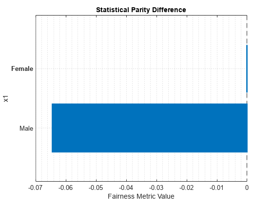
For the nonreference group (Male), the SPD value is the difference between the probability of a patient being in the positive class (Nonsmoker) when the sensitive attribute value is Male and the probability of a patient being in the positive class when the sensitive attribute value is Female (in the reference group). Ideally, SPD values are close to 0.
To try to improve the nonreference group SPD value, you can adjust the model predictions by using the fairnessThresholder function. The function searches for an optimal score threshold to maximize accuracy while satisfying fairness bounds. For observations in the critical region below the optimal threshold, the function changes the labels so that the fairness constraints hold for the reference and nonreference groups. By default, when you use the SPD bias metric, the function tries to find a score threshold such that the SPD value for the nonreference group is in the range [–0.05,0.05].
fairnessMdl = fairnessThresholder(mdl,validationX, ...
    validationAttribute,validationY, ...
    BiasMetric="StatisticalParityDifference")
fairnessMdl =
  fairnessThresholder with properties:

               Learner: [1×1 classreg.learning.classif.CompactClassificationSVM]
    SensitiveAttribute: [50×1 categorical]
       ReferenceGroups: Female
          ResponseName: 'Y'
         PositiveClass: Nonsmoker
        ScoreThreshold: 0.5116
            BiasMetric: 'StatisticalParityDifference'
       BiasMetricValue: -0.0209
       BiasMetricRange: [-0.0500 0.0500]
        ValidationLoss: 0.1200
fairnessMdl is a fairnessThresholder model object.
Note that the updated nonreference group SPD value is closer to 0.
newNonReferenceSPD = fairnessMdl.BiasMetricValue
newNonReferenceSPD =
-0.0209
Use the new score threshold to adjust the validation data predictions. The predict function of the fairnessMdl object adjusts the prediction of each observation whose maximum score is less than the score threshold. If the observation is in the nonreference group, the function predicts the observation into the positive class. If the observation is in the reference group, the function predicts the observation into the negative class. These adjustments do not always result in a change in the predicted label.
fairnessLabels = predict(fairnessMdl,validationX, ...
    validationAttribute);
Find the observations whose predictions are switched by fairnessMdl.
differentIdx = (labels ~= fairnessLabels);
differentX = validationX(differentIdx,:);
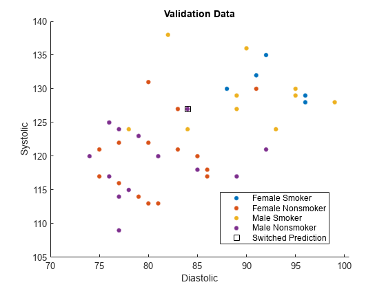
names(5) = "Switched Prediction";Plot the validation data. The color of each point indicates the sensitive attribute group and class label for that observation. Points in squares indicate observations whose labels are switched by the fairnessThresholder model.
figure
hold on
gscatter(validationX(:,1),validationX(:,2), ...
    validationAttribute.*validationY)
plot(differentX(:,1),differentX(:,2), ...
    "ks",MarkerSize=8)
legend(names)
xlabel("Diastolic")
ylabel("Systolic")
title("Validation Data")
hold off
The fairnessThresholder function uses a technique designed for binary sensitive attributes that contain a reference group and a nonreference group. This example shows how to use the function when the sensitive attribute contains more than two groups.
Read the sample file CreditRating_Historical.dat into a table. The predictor data contains financial ratios for a list of corporate customers. The response variable contains credit ratings assigned by a rating agency. Consider the industry sector information as a sensitive attribute.
creditrating = readtable("CreditRating_Historical.dat");Because each value in the ID variable is a unique customer ID—that is, length(unique(creditrating.ID)) is equal to the number of observations in creditrating—the ID variable is a poor predictor. Remove the ID variable from the table, and convert the Industry variable to a categorical variable.
creditrating.ID = [];
creditrating.Industry = categorical(creditrating.Industry);
In the Rating response variable, combine the AAA, AA, A, and BBB ratings into a category of "good" ratings, and the BB, B, and CCC ratings into a category of "poor" ratings.
Rating = categorical(creditrating.Rating);
Rating = mergecats(Rating,["AAA","AA","A","BBB"],"good");
Rating = mergecats(Rating,["BB","B","CCC"],"poor");
creditrating.Rating = Rating;
Partition the data into a training set, validation set, and test set. Use approximately one third of the observations to create each set.
rng("default")
cv1 = cvpartition(creditrating.Rating,"Holdout",1/3);
tblNotForTest = creditrating(training(cv1),:);
tblTest = creditrating(test(cv1),:);

cv2 = cvpartition(tblNotForTest.Rating,"Holdout",1/2);
tblTrain = tblNotForTest(training(cv2),:);
tblValidation = tblNotForTest(test(cv2),:);
In this example, consider industries with high ratios of good to poor ratings as reference groups in the Industry sensitive attribute. Compute the ratios using the training data set tblTrain and the grpstats function.
info = grpstats(tblTrain,["Industry","Rating"]);
goodInfo = info(info.Rating == "good",1:3);
poorInfo = info(info.Rating == "poor",1:3);
goodToPoorRatio = goodInfo.GroupCount./poorInfo.GroupCount
goodToPoorRatio = 12×1

    2.0000
    1.5122
    2.1212
    1.3061
    1.7778
    2.5152
    2.4118
    1.9394
    1.4186
    1.1875
    2.8846
    2.1667
Define the well-rated industries as those with goodToPoorRatio values greater than 2.5. Consider the industry with the highest goodToPoorRatio value as the best-rated industry.
wellRatedIndustries = goodInfo.Industry(goodToPoorRatio > 2.5,:)
wellRatedIndustries = 2×1 categorical
     6
     11
maximumRatio = max(goodToPoorRatio);
bestRatedIndustry = goodInfo.Industry(goodToPoorRatio == maximumRatio,:)
bestRatedIndustry = categorical
     11
Compute fairness metrics with respect to the sensitive attribute by using the training data. In particular, find the statistical parity difference (SPD) for each group in Industry. Specify a good rating as the positive class, and specify the best-rated industry (11) as the reference group. Use the report and plot object functions of fairnessMetrics to display the results.
dataMetricsResults = fairnessMetrics(tblTrain,"Rating", ...
    SensitiveAttributeNames="Industry", ...
    PositiveClass="good",ReferenceGroup=bestRatedIndustry);
report(dataMetricsResults,BiasMetrics="StatisticalParityDifference")
ans=12×3 table
    SensitiveAttributeNames    Groups    StatisticalParityDifference
    _______________________    ______    ___________________________

           Industry              1                -0.075908
           Industry              2                 -0.14063
           Industry              3                -0.062963
           Industry              4                  -0.1762
           Industry              5                 -0.10257
           Industry              6                -0.027057
           Industry              7                -0.035678
           Industry              8                 -0.08278
           Industry              9                 -0.15604
           Industry              10                -0.19972
           Industry              11                       0
           Industry              12               -0.058364
plot(dataMetricsResults,"StatisticalParityDifference")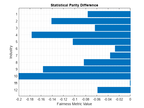
For each group g in the sensitive attribute, the SPD value is the difference between the probability of being in the positive class (good) when the sensitive attribute value is g and the probability of being in the positive class when the sensitive attribute value is the reference group value (11). Ideally, SPD values are close to 0.
Visualize the distribution of SPD values by using a box plot.
boxchart(dataMetricsResults.BiasMetrics.StatisticalParityDifference)
ylabel("Statistical Parity Difference")
legend("Training Data")
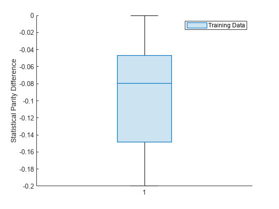
The median SPD value is around –0.08.
Train a binary tree classifier using the training data set. Use the trained model to predict labels and compute the classification error on the test data set.
predictorNames = ["WC_TA","RE_TA","EBIT_TA","MVE_BVTD","S_TA"];
treeMdl = fitctree(tblTrain,"Rating", ...
    PredictorNames=predictorNames);
treePredictions = predict(treeMdl,tblTest);
L = loss(treeMdl,tblTest)
L =
0.1107
You can adjust model predictions by using the fairnessThresholder function. The function uses the validation data to search for an optimal score threshold that maximizes accuracy while satisfying fairness bounds. Use the ReferenceGroups name-value argument to specify the well-rated industries (6 and 11) as the reference group. All other industries form the nonreference group. Specify the bias metric as the statistical parity difference and the bias metric range as [–0.005,0.005]. Note that these bounds apply to the SPD value for the collective nonreference group, not individual industries in the sensitive attribute.
fairnessMdl = fairnessThresholder(treeMdl,tblValidation, ...
"Industry","Rating", ...
PositiveClass="good",ReferenceGroups=wellRatedIndustries, ...
BiasMetric="StatisticalParityDifference", ...
BiasMetricRange=[-0.005 0.005])
fairnessMdl =
  fairnessThresholder with properties:

               Learner: [1×1 classreg.learning.classif.CompactClassificationTree]
    SensitiveAttribute: 'Industry'
       ReferenceGroups: [2×1 categorical]
          ResponseName: 'Rating'
         PositiveClass: 'good'
        ScoreThreshold: 0.5444
            BiasMetric: 'StatisticalParityDifference'
       BiasMetricValue: 0.0034
       BiasMetricRange: [-0.0050 0.0050]
        ValidationLoss: 0.1198
fairnessMdl is a fairnessThresholder model object.
Adjust the test set predictions by using the new score threshold, and calculate the classification error.
newPredictions = predict(fairnessMdl,tblTest);
newL = loss(fairnessMdl,tblTest)
newL =
0.1183
The new classification error is similar to the original classification error.
Compare the SPD values across the two sets of test predictions: the original predictions computed using treeMdl and the adjusted predictions computed using fairnessMdl. Specify a good rating as the positive class, and specify the best-rated industry (11) as the reference group. Use the report and plot object functions of fairnessMetrics to display the results.
predMetricsResults = fairnessMetrics(tblTest,"Rating", ...
    SensitiveAttributeNames="Industry", ...
    Predictions=[treePredictions,newPredictions], ...
    PositiveClass="good", ...
    ModelNames=["Original Model","Adjusted Model"], ...
    ReferenceGroup=bestRatedIndustry);
report(predMetricsResults,BiasMetric="DisparateImpact")
ans=12×5 table
        Metrics        SensitiveAttributeNames    Groups    Original Model    Adjusted Model
    _______________    _______________________    ______    ______________    ______________

    DisparateImpact           Industry              1          0.96499           0.95014
    DisparateImpact           Industry              2           1.0755            1.0634
    DisparateImpact           Industry              3          0.94643           0.94643
    DisparateImpact           Industry              4           1.0541            1.0392
    DisparateImpact           Industry              5           1.0262            1.0132
    DisparateImpact           Industry              6           1.0186            1.0186
    DisparateImpact           Industry              7          0.99692           0.96067
    DisparateImpact           Industry              8            1.077             1.077
    DisparateImpact           Industry              9           1.0392            1.0103
    DisparateImpact           Industry              10          1.0781            1.0635
    DisparateImpact           Industry              11               1                 1
    DisparateImpact           Industry              12          1.0392            1.0225
plot(predMetricsResults,"spd")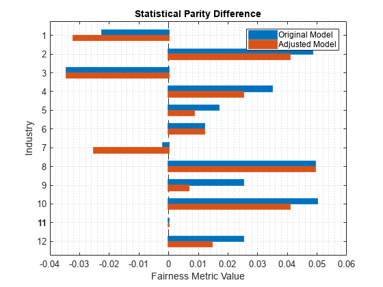
Visualize the two distributions of SPD values by using box plots.
boxchart(predMetricsResults.BiasMetrics.StatisticalParityDifference, ...
GroupByColor=predMetricsResults.BiasMetrics.ModelNames)
ylabel("Statistical Parity Difference")
legend
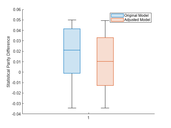
The SPD values for the original test set predictions are close to 0, with a median value of approximately 0.02. The SPD values for the adjusted test set predictions have a median value that is slightly closer to 0.
Train a logistic regression model using the fitglm function. To adjust the score threshold for classifying observations, pass the model as an input to fairnessThresholder using a function handle.
Load the patients data set, which contains medical information for 100 patients. Convert the Gender and Smoker variables to categorical variables. Specify the descriptive category names Smoker and Nonsmoker rather than 1 and 0.
load patients
Gender = categorical(Gender);
Smoker = categorical(Smoker,logical([1 0]), ...
    ["Smoker","Nonsmoker"]);
Create a table containing the continuous predictors Diastolic and Systolic, the sensitive attribute Gender, and the response variable Smoker.
Tbl = table(Diastolic,Systolic,Gender,Smoker);
Partition the data into training and validation sets. Use half of the observations for training and half of the observations for validation.
rng("default") % For reproducibility
cv = cvpartition(Tbl.Smoker,"Holdout",0.5);
trainTbl = Tbl(training(cv),:);
validationTbl = Tbl(test(cv),:);
Train a logistic regression model using the training data trainTbl and the fitglm function.
modelspec = "Smoker ~ Diastolic + Systolic";
glmMdl = fitglm(trainTbl,modelspec,Distribution="binomial")
glmMdl =
Generalized linear regression model:
    logit(P(Smoker='Nonsmoker')) ~ 1 + Diastolic + Systolic
    Distribution = Binomial

Estimated Coefficients:
                   Estimate      SE        tStat      pValue
                   ________    _______    _______    _________

    (Intercept)      116.98     44.939     2.6032    0.0092356
    Diastolic      -0.54261    0.21577    -2.5147     0.011913
    Systolic       -0.57999    0.28697    -2.0211     0.043268


50 observations, 47 error degrees of freedom
Dispersion: 1
Chi^2-statistic vs. constant model: 54, p-value = 1.89e-12
As indicated in the linear regression model equation, Nonsmoker is the positive class. That is, an observation with a predicted score greater than 0.5 is predicted to be a nonsmoker.
Create a function handle to the predict function of the GeneralizedLinearModel object glmMdl.
f = @(T) predict(glmMdl,T);
Create a fairnessThresholder object by using the function handle f and the validation data validationTbl. The function searches for an optimal score threshold to maximize accuracy while satisfying fairness bounds. Specify the bias metric range so that the disparate impact value for the nonreference group is in the range [0.9,1.1].
When you pass a classification model as a function handle, you must specify the positive class.
fairnessMdl = fairnessThresholder(f,validationTbl, ...
    "Gender","Smoker", ...
    BiasMetricRange=[0.9 1.1], ...
    PositiveClass=categorical("Nonsmoker"))
fairnessMdl =
  fairnessThresholder with properties:

               Learner: @(T)predict(glmMdl,T)
    SensitiveAttribute: 'Gender'
       ReferenceGroups: Female
          ResponseName: 'Smoker'
         PositiveClass: Nonsmoker
        ScoreThreshold: 0.8087
            BiasMetric: 'DisparateImpact'
       BiasMetricValue: 0.9538
       BiasMetricRange: [0.9000 1.1000]
        ValidationLoss: 0.1600
omega = fairnessMdl.ScoreThreshold
omega =
0.8087
fairnessMdl is a fairnessThresholder model object. For each observation with a score in the range (1–omega,omega), the predict function of the fairnessMdl object adjusts the prediction. If the observation is in the nonreference group (Male), the function predicts the observation into the positive class (Nonsmoker). If the observation is in the reference group (Female), the function predicts the observation into the negative class (Smoker).
Adjust the predictions for the entire data set Tbl by using the new score threshold.
fairnessLabels = predict(fairnessMdl,Tbl)
fairnessLabels = 100×1 categorical
     Smoker
     Nonsmoker
     Smoker
     Nonsmoker
     Nonsmoker
     Nonsmoker
     Smoker
     Nonsmoker
     Nonsmoker
     Nonsmoker
     Nonsmoker
     Nonsmoker
     Nonsmoker
     Smoker
     Nonsmoker
     Smoker
     Smoker
     Nonsmoker
     Nonsmoker
     Nonsmoker
     Nonsmoker
     Nonsmoker
     Nonsmoker
     Smoker
     Smoker
     Nonsmoker
     Nonsmoker
     Nonsmoker
     Nonsmoker
     Smoker
      ⋮
Algorithms
References
[1] Kamiran, Faisal, Asim Karim, and Xiangliang Zhang. "Decision Theory for Discrimination-Aware Classification." 2012 IEEE 12th International Conference on Data Mining: 924-929.
Version History
Introduced in R2023a