Résultats pour
MATLAB EXPO India | 7 May | Bengaluru
Get inspired by the latest trends and real-world customer success stories transforming industries. Learn from trusted experts across 4 tracks.
- AI & Autonomous Systems
- Electrification
- Systems & Software Engineering
- Radar, Wireless & HDL
Register at bit.ly/matlabexpocommunity

Do we know if MATLAB is being used on the Artemis II (moon mission) spacecraft itself? Like is the crew running MATLAB programs? I imagine it was probably at least used in development of some of the components of the spacecraft, rockets, or launch building. Or is it used for any of the image analysis of the images collected by the spacecraft?
MATLAB interprets the first block of uninterupted comments in a function file as documentation. Consider a simple example.
% myfunc This is my function
%
% See also sin
function z = myfunc(x, y)
z = x + y;
end
Those comments are printed in the command window with "help myfunc" and displayed in a separate window with "doc myfunc". A lot of useful things happen behind the scenes as well.
- Hyperlinks are automatically added for valid file names after "See also".
- When dealing with classes, the doc command automatically appends the comment block with a lists of properties and methods.
All this is very handy and as been around for quite some time. However, the doc browser isn't great (forward/back feature was removed several versons ago), the text formatting isn't great, and there is no way to display math.
Although pretty text/math can be displayed in a live document, the traditional *.mlx file format does not always play nice with Git and I have avoided them. However, live documents can now (since 2025a?) be saved in a pure text format, so I began to wonder if all functions should be written in this style. Turns out that all you have to do is append these lines:
%[appendix]{"version":"1.0"}
%---
to the end of any function file to make it a live function. Doing so changes how MATLAB manages that first comment block. The help command seems to be unaffacted, although [text] may appear at the start of each comment line (depending on if the file was create as a live function or subsequently converted). The doc command behaves very different: instead of bringing up the traditional window for custom documentation, the comment block looks like it gets published to HTML and looks more similar to standard MATLAB help. This is a win in some ways, but the "See also" capabilitity is lost.
Curiously, the same text can be appended to the end of a class definition file with some affect. It does not change how the file shows up in the editor, but as in live functions, comments are published when using the doc command. So we are partway to something like a "live class", but not quite.
Should one stick with traditional *.m files or make everything live? Neither does a great job for functions/classes in a namespace--references must explicitly know absolute location in traditional functions, and there is no "See also" concept in a live function. Do we need a command, like cdoc (custom documentation), that pulls out the comment block, publishing formatted text to HTML while simultaneously resolving "See also" references as hyperlinks? If so, it would be great if there were other special commands like "See examples" that would automatically copy and then open an example script for the end user.
Hi all,
I'm a UX researcher here at MathWorks working on the MathWorks Central Community. We're testing a new feature to make it easier to ask a question, and we'd love to hear from community members like you.
Sessions will be next week. They are remote, up to 2 hours (often shorter), and participants receive a $100 stipend. If you're interested, you can click here to schedule.
Thanks in advance! Your feedback directly shapes what gets built.
--David, MathWorks UX Research
Digital Twin Development of PEARL Autonomous Surface System Thermal Management
The top session of the countdown showcases how the PEARL engineering team used a digital twin to solve real‑world thermal challenges in a solar‑powered autonomous marine platform operating in extreme environments. After thermal shutdown events in the field, the team built a model that predicts temperatures at multiple locations with ~1% accuracy, while balancing accuracy with model complexity.
Beyond the technology, this keynote delivers practical lessons for predictive modeling and digital twins that apply well beyond marine systems.
We hope you’ve enjoyed the Top 10 countdown series—and a big thank‑you to Olivier de Weck at Massachusetts Institute of Technology, for delivering such a compelling and insightful keynote.
🎥 If you missed it live, be sure to watch the recording to see why it earned the #1 spot at MATLAB EXPO 2026.

MATLAB EXPO India is Back!
This in-person events brings together engineers, scientists, and researchers to explore the latest trends in engineering and science, and discover new MATLAB and Simulink capabilities to apply to your work.
May 7, 2026 l Bengaluru
Register at bit.ly/matlabexpocommunity

It’s no surprise this keynote landed at #2. MaryAnn Freeman, Senior Director of Engineering, AI, and Data Science explores how AI, especially generative AI, is transforming the way engineers design, build, and innovate. From accelerating the design loop with faster, data‑driven solutions, to blending human creativity with AI insights, to evolving engineering tools that turn ideas into build‑ready systems. This keynote shows how embedded intelligence helps engineers push past traditional limits and bridge imagination with real‑world impact.
If you’re curious about how AI is reshaping engineering workflows today (and what that means for the future of design), this is a must‑watch.
👉 Watch the keynote recording and see why it was one of the most popular sessions of MATLAB EXPO Online 2025.
Absolutely!
65%
Probably
9%
Sometimes yes, sometimes no
4%
Unlikely
17%
Never!
4%
23 votes
Matlab seems to follow a rule that iterative reduction operators give appropriate non-empty values to empty inputs. Examples include,
sum([])
prod([])
all([])
any([])
Is it an oversight not to do something similar for min and max?
max([])
For non-empty A and B,
max([A,B])= max(max(A), max(B))
The extension to B=[] should therefore satisfy,
max(A)=max(max(A),max([]))
for any A, which will only be true if we define max([])=-inf.
The 550,000th question has been asked on Answers.
Software‑defined vehicles are becoming reality—and this #3 ranked session shows how. In this keynote, Daniel Scurtu (NXP) demonstrates how MathWorks and NXP are working together to accelerate system‑level embedded development.
🔋 Using a vehicle electrification demo that runs across multiple NXP processors, you’ll see:
- Model‑Based Design workflows from concept to deployment
- Intelligent battery management and motor control
- Automatic code generation and hardware deployment
- ☁️ Real‑time cloud analytics and over‑the‑air updates
🛠️ Featuring MATLAB and Simulink products alongside NXP tools like Model-based Design Toolbox (MBDT), S32 Design Studio IDE, and Real-Time Drivers (RTD), this session highlights an end‑to‑end approach that reduces complexity and speeds the transition to software‑defined vehicles.
If you have published add-ons on File Exchange, you may have noticed that we recently added a new, unique package name field to all add-ons. This enables future support for automated installation with the MATLAB Package Manager. This name will be a unique identifier for your add-on and does not affect the existing add-on title, any file names, or the URL of your add-on.
📝 Update and review until April 10
We generated default package names for all add-ons. You can review and update the package name for your add-ons until April 10, 2026. Review your package names now:
After April 10, you will need to create a new version to change your package name.
🚀 More changes coming with the MATLAB R2026b prerelease
Starting with the MATLAB R2026b prerelease, these package names will take effect. At that time, the package name may appear on the File Exchange page for your add-on.
Keep your eyes peeled for exciting changes coming soon to your add-ons on File Exchange!
Cantera is an open-source suite of tools for problems involving chemical kinetics, thermodynamics, and transport processes. Dr. Su Sun, a recent graduate from Northeastern Chemical Engineering Ph.D. program made significant contributions to MATLAB interface for Cantera in Cantera Release 3.2.0 in collaboration with Dr. Richard West, other Cantera developers, and MathWorks Advanced Support and Development Teams. As part of this Release, MATLAB interface for Cantera transitioned to using the new MATLAB- C++ interface and expanded their unit testing. Further information is available here.
I began coding in MATLAB less than 2 months ago for a class at community college. Alongside the course content, I also completed the MATLAB onramp and introduction to linear algebra self-paced online courses. I think this is the most fun I've had coding since back when I used to make Scratch projects in elementary school. I'm kind of curious if I could recreate some of my favorite childhood Scratch games here.
Anyways, I just wanted to introduce myself since I plan to be really active this year. My name is Mehreen (meh like the meh emoji from the Emoji movie, reen like screen), I'm a data science undergrad sophomore from the U.S. and it's nice to meet you!
What’s New in MATLAB and Simulink in 2025
If you missed this session live, this is one of those “everyone’s talking about it” updates you’ll want to catch up on. 👀
This session is packed with the kinds of enhancements that quietly (and not so quietly) change how you work every day.
Here’s why it earned a spot in our Top 4:
- A redesigned MATLAB desktop with customizable sidebars and light/dark themes—built to adapt to how you work
- New side panels for coding and development tasks, plus more control over organizing and customizing figures
- MATLAB Copilot, a generative AI assistant optimized for MATLAB to help you explore ideas, learn techniques, and boost productivity directly in the desktop
- Simulink workflow improvements like a redesigned Simulink scope, more detailed info in quick insert, and automatic signal line straightening
- Enhanced Python integration across MATLAB and Simulink
- New AI deployment options optimized for Qualcomm and Infineon hardware targets
If staying current with MATLAB and Simulink is part of your role—or your edge—this session is a must‑watch. Missing it means missing context for features that will shape how you work in 2026 and beyond.
💬 Discussion topic:
Which single update from this release do you think will most improve your day‑to‑day workflow, and why?
An emirp is a prime that is prime when viewed in in both directions. They are not too difficult to find at a lower level. For example...
isprime([199 991])
Gosh, that was easy. But what happens if the number is a bit larger? The problem is, primes themselves tend to be rare on the number line when you get into thousands or tens of thousands of decimal digits. And recently, I read that a world record size prime had been found in this form. You have probably all heard of Matt Parker and numberphile.
And so, I decided that MATLAB would be capable of doing better. Why not? After all, at the time, the record size emirp had only 10002 decimal digits.
How would I solve this problem? First, we can very simply write a potential emirp as
10^n + a
then we can form the flipped version as
ahat*10^(n-d) + 1
where ahat is the decimally flipped version of a, and d is chosen based on the number of decimal digits in the number a itself. Not all emirps will be of that form of course, but using all of those powers of 10 makes it easy to construct a large number and its reversed form. And that is a huge benefit in this. For example,
Pfor = sym(10)^101 + 943
Prev = 349*sym(10)^99 + 1
It is easier to view these numbers using a little code I wrote, one that redacts most of those boring zeros.
emirpdisplay(Pfor)
emirpdisplay(Prev)
And yes, they are both prime, and they both have 102 decimal digits.
isprime([Pfor,Prev])
Sadly, even numbers that large are very small potatoes, at least in the world of large primes. So how do we solve for a much larger prime pair using MATLAB?
The first thing I want to do is to employ roughness at a high level. If a number is prime, then it is maximally rough. (I posted a few discussions about roughness some time ago.)
https://www.mathworks.com/matlabcentral/discussions/tips/879745-primes-and-rough-numbers-basic-ideas
In this case, I'm going to look for serious roughness, thus 2e9-rough numbers. Again, a number is k-rough if its smallest prime factor is greater than k. There are roughly 98 million primes below 2e9.
The general idea is to compute the remainders of 10^12345, modulo every prime in that set of primes below 2e9. This MUST be done using int64 or uint64 arithmetic, as doubles will start to fail you above
format short g
sqrt(flintmax)
The sqrt is in there because we will be multiplying numbers together here, and we need always to stay below intmax for the integer format you are working with. However, if we work in an integer format, we can get as high as 2e9 easily enough, by going to int64 or uint64.
sqrt(double(intmax('int64')))
And, yes, this means I could have gone as high as primes(3e9), however, I stopped at 2e9 due to the amount of RAM on my computer. 98 million primes seemed enough for this task. And even then, I found myself working with all of the cores on my computer. (Note that I found int64 arithmetic will only fire up the performance cores on your Mac via automatic multi-threading. Mine has 12 performance cores, even though it has 16 total cores.)
I computed the remainders of 10^12345 with respect to each prime in that set using a variation of the powermod algorithm. (Not powermod itself, which was itself not sufficiently fast for my purposes.) Once I had those 98 millin remainders in a vector, then it became easy to use a variation of the sieve of Eratosthenes to identify 2e9-rough numbers.
For example, working at 101 decimal digits, if I search for primes of the form 10^101+a, with a in the interval [1,10000], there are 256 numbers of that form which are 2e9-rough. Roughness is a HUGE benefit, since as you can see here, I would not want to test for primality all 10000 possible integers from that interval.
Next, I flip those 256 rough numbers into their mirror image form. Which members of that set are also rough in the mirror image form? We would then see this further reduces the set to only 34 candidates we need test for primality which were rough in both directions. With now only a few direct tests for primality, we would find that pair of 102 digit primes shown above.
Of course, I'm still needing to work with primes in the regime of 10000 plus decimal digits, and that means I need to be smarter about how I test a number to be prime. The isprime test given by sym/isprime only survives out to around 1000 decimal digits before it starts to get too slow. That means I need to perform Fermat tests to screen numbers for primality. If that indicates potential primality, I currently use a Miller-Rabin code to verify that result, one based on the tool Java.Math.BigInteger.isProbablePrime.
And since Wikipedia tells me the current world record known emirp was
117,954,861 * 10^11111 + 1 discovered by Mykola Kamenyuk
that tells me I need to look further out yet. I chose an exponent of 12345, so starting at 10^12345. Last night I set my Mac to work, with all cores a-fumbling, a-rumbling at the task as I slept. Around 4 am this morning, it found this number:
emirp = @(N,a) sym(10)^N + a;
Pfor = emirp(12345,10519197);
Prev = sym(flip(char(Pfor)));
emirpdisplay(Pfor)
emirpdisplay(Prev)
isProbablePrimeFLT([Pfor,Prev],210)
I'm afraid you will need to take my word for it that both also satisfy a more robust test of primality, as even a Miller-Rabin test that will take more time than the MATLAB version we get for use in a discussion will allow. As far as a better test in the form of the MATLAB isprime utility to verify true primality, that test is still running on my computer. I'll check back in a few hours to see if it fininshed.
Anyway, the above numbers now form the new world record known emirp pair, at 12346 decimal digits. Yes, I do recognize this is still what I would call low hanging fruit, that having announced a largest prime of this form, someone else willl find one yet larger in a few weeks or months. But even so, for the moment, MATLAB owns the world record!
If anyone else wants a version of the codes I used for the search, I've attached a version (emirpsearchpar.m) that employs the parallel processing toolbox. I do have as well a serial version which is of course, much, much slower. It would be fun to crowd source a larger world record yet from the MATLAB community.
Hey folks in MATLAB community! I'm an engineering student from India messing around with deep learning/ML for spotting faults in power electronics stuff—like inverter issues or microgrid glitches in Simulink.
What's your take?
- Which toolbox rocks for this—Deep Learning one or Predictive Maintenance?
- Any gotchas when training on sim data vs real hardware?
- Cool workflows or GitHub links you've used?
Would love your real experiences! 😊
🤖 What does it take to make robotic motion feel… human?
In this session, Tetsushi Sotowa shares how NSK is combining advanced control techniques with deep learning to enable human‑like grasping in electric grippers
You’ll see a real‑world case study featuring:
- Bilateral and force control systems developed in‑house
- MATLAB and Simulink–based control workflows
- Deep learning integration using Deep Learning Toolbox
- A practical path from mechatronics research to intelligent actuation
The result: an AI‑enhanced actuator capable of more natural, responsive grasping—bringing robotics one step closer to human motion.
👉 Interested in AI‑driven robotics and advanced control? Check out the session now from MATLAB EXPO 2025.
The "Issues" with Constant Properties
MATLABs Constant properties can be rather difficult to deal with at times. For those unfamiliar there are two distinct behaviors when accessing constant properties of a class. If a "static" pattern is used ClassName.PropName the the value, as it was assigned to the property is returned; that is to say that you will have a nargout of 1. But, rather frustratingly, if an instance of the class is used when accessing the constant property, such as ArrayOfClassName.PropName then your nargout will be equivalent to the number of elements in the array; this means that functionally the constant property accessing scheme is identical to that of the element wise properties you find on "instance" properties.
Motivation for Correcting Constant Property Behavior
This can be frustraing since constant properties are conceptually designed to tie data to a class. You could see this design pattern being useful where a super class were to define an abstract constant property, that would drive the behavior of subclasses; the subclasses define the value of the property and the super class uses it. I would like to use this design to develop a custom display "MatrixDisplay" focused mixin (like the internal matlab.mixin.internal.MatrixDisplay). The idea is that missing element labels, invalid handle element labels, and other semantic values can be configured by the subclasses, conveniently just by setting the constant properties; these properties will be used by the super class to substitute the display strings of appropriate elements. Most of the processing will happen within the super class as to enable simple, low-investment, opt-in display options for array style classes.
The issue is that you can not rely on constant property access to return the appropriate value when the instance you've been passed is empty. This also happens with excessive outputs when the instance is non-scalar, but those extra values from the CSL are just ignored, while Id imagine there is an effect on performance from generating the excess outputs (assuming theres no internal optimization for the unused outputs), this case still functions appropriately. As I enjoying exploring MATLAB, I found an internal indexing mixing class in the past that provides far greater control of do indexing; I've done a good deal of neat things with it, though at the cost of great overhead when getting implementing cool "proof of concept/showcase" examples. Today I used it to quickly implement a mix in that "fixes" constant properties such that they always return as though they were called statically from the class name, as opposed to an instance.
A Simplistic Solution
To do this I just intercepted the property indexing, checked if it was constant, and used the DefaultValue property of the metadata to return the value. This works nicely since we are required to attempt to initialize a "dummy" scalar array, or generate a function handle; both of those would likely be slower, and in the former case, may not be possible depending on the subclass implementation. It is worth noting that this method of querying the value from metadata is safe because constant properties are immutable and thus must be established as the class is loaded. Below is the small utility class I have implemented to get predictable constant variable access into classes that benefit from it. Lastly it is worth noting that I've not torture testing the rerouting of the indexing we aren't intercepting, in my limited play its behaved as expected but it may be worth looking over if you end up playing around with this and notice abnormal property assignment or reading from non-constant properties.
Sample Class Implementation
classdef(Abstract, HandleCompatible) ConstantProperty < matlab.mixin.internal.indexing.RedefinesDotProperties
%ConstantProperty Returns instance indexed constant properties as though they were statically indexed.
% This class overloads property access to check if the indexed property is constant and return it properly.
%% Property membership utility methods
methods(Access=private)
function [isConst, isProp] = isConstantProp(obj, prop, options)
%isConstantProp Determine if the input property names are constant properties of the input
arguments
obj mixin.ConstantProperty;
prop string;
options.Flatten (1, 1) logical = false;
end
% Store the cache to avoid rechecking string membership and parsing metadata
persistent class_cache
% Initialize cache for all subclasses to maintain their own caches
if(isempty(class_cache))
class_cache = configureDictionary("string", "dictionary");
end
% Gather the current class being analyzed
classname = string(class(obj));
% Check if the current class has a cache, if not make one
if(~isKey(class_cache, classname))
class_cache(classname) = configureDictionary("string", "struct");
end
% Alias the current classes cache
prop_cache = class_cache(classname);
% Check which inputs are already cached
isCached = isKey(prop_cache, prop);
% Add any values that have yet to be cached to the cache
if(any(~isCached, "all"))
% Flatten cache additions
props = row(prop(~isCached));
% Gather the meta-property data of the input object and determine if inputs are listed properties
mc_props = metaclass(obj).PropertyList;
% Determine which properties are keys
[isConst, idx] = ismember(props, string({mc_props.Name}));
idx = idx(isConst);
% Check which of the inputs are constant properties
isConst = repmat(isConst, 2, 1);
isConst(1, isConst(1, :)) = [mc_props(idx).Constant];
% Parse the results into structs for caching
cache_values = cell2struct(num2cell(isConst), ["isConst"; "isProp"]);
prop_cache(props) = row(cache_values);
% Re-sync the cache
class_cache(classname) = prop_cache;
end
% Extract results from the cache
values = prop_cache(prop);
if(options.Flatten)
% Split and reshape output data
sz = size(prop);
isConst = reshape(values.isConst, sz);
isProp = reshape(values.isProp, sz);
else
isConst = struct2cell(values);
end
end
function [isConst, isProp] = isConstantIdxOp(obj, idxOp)
%isConstantIdxOp Determines if the idxOp is referencing a constant property.
arguments
obj mixin.ConstantProperty;
idxOp (1, :) matlab.indexing.IndexingOperation;
end
import matlab.indexing.IndexingOperationType;
if(idxOp(1).Type == IndexingOperationType.Dot)
[isConst, isProp] = isConstantProp(obj, idxOp(1).Name);
else
[isConst, isProp] = deal(false);
end
end
function A = getConstantProperty(obj, idxOp)
%getConstantProperty Returns the value of a constant property using a static reference pattern.
arguments
obj mixin.ConstantProperty;
idxOp (1, :) matlab.indexing.IndexingOperation;
end
A = findobj(metaclass(obj).PropertyList, "Name", idxOp(1).Name).DefaultValue;
end
end
%% Dot indexing methods
methods(Access = protected)
function A = dotReference(obj, idxOp)
arguments(Input)
obj mixin.ConstantProperty;
idxOp (1, :) matlab.indexing.IndexingOperation;
end
arguments(Output, Repeating)
A
end
% Force at least one output
N = max(1, nargout);
% Check if the indexing operation is a property, and if that property is constant
[isConst, isProp] = isConstantIdxOp(obj, idxOp);
if(~isProp)
% Error on invalid properties
throw(MException( ...
"JB:mixin:ConstantProperty:UnrecognizedProperty", ...
"Unrecognized property '%s'.", ...
idxOp(1).Name ...
));
elseif(isConst)
% Handle forwarding indexing operations
if(isscalar(idxOp))
% Direct assignment
[A{1:N}] = getConstantProperty(obj, idxOp);
else
% First extract constant property then forward indexing operations
tmp = getConstantProperty(obj, idxOp);
[A{1:N}] = tmp.(idxOp(2:end));
end
else
% Handle forwarding indexing operations
if(isscalar(idxOp))
% Unfortunately we can't just recall obj.(idxOp) to use default/built-in so we manually extract
[A{1:N}] = obj.(idxOp.Name);
else
% Otherwise let built-in handling proceed
tmp = obj.(idxOp(1).Name);
[A{1:N}] = tmp.(idxOp(2:end));
end
end
end
function obj = dotAssign(obj, idxOp, values)
arguments(Input)
obj mixin.ConstantProperty;
idxOp (1, :) matlab.indexing.IndexingOperation;
end
arguments(Input, Repeating)
values
end
% Handle assignment based on presence of forward indexing
if(isscalar(idxOp))
% Simple broadcasted assignment
[obj.(idxOp.Name)] = deal(values{:});
else
% Initialize the intermediate values and expand the values for assignment
tmp = {obj.(idxOp(1).Name)};
[tmp.(idxOp(2:end))] = deal(values{:});
% Reassign the modified data to the output object
[obj.(idxOp(1).Name)] = deal(tmp{:});
end
end
function n = dotListLength(obj, idxOp, idxCnt)
arguments(Input)
obj mixin.ConstantProperty;
idxOp (1, :) matlab.indexing.IndexingOperation;
idxCnt (1, :) matlab.indexing.IndexingContext;
end
if(isConstantIdxOp(obj, idxOp))
if(isscalar(idxOp))
% Constant properties will also be 1
n = 1;
else
% Checking forwarded indexing operations on the scalar constant property
n = listLength(obj.(idxOp(1).Name), idxOp(2:end), idxCnt);
end
else
% Check the indexing operation normally
% n = listLength(obj, idxOp, idxCnt);
n = numel(obj);
end
end
end
end
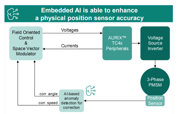
Missed a crowd‑favorite session feautring Marko Gecic at Infineon and Lucas Garcia at MathWorks?
This talk shows how to verify and test AI for real‑time, safety‑critical systems using an AI virtual sensor that estimates motor rotor position on an Infineon AURIX TC4x microcontroller. Built with MATLAB and Simulink, the demo covers training, verification, and real‑time control across a wide range of operating conditions.
You’ll see practical techniques to test robustness, measure sensitivity to input perturbations, and detect out‑of‑distribution behavior—critical steps for meeting standards like ISO 26262 and ISO 8800. The session also highlights how Model‑Based Design leverages AURIX TC4x features such as the PPU and CDSP to deploy AI with confidence.