How to Design an MPC Controller with Simulink and Model Predictive Control Toolbox | Understanding Model Predictive Control, Part 6
From the series: Understanding Model Predictive Control
Melda Ulusoy, MathWorks
Learn how to design an MPC controller for an autonomous vehicle steering system using Model Predictive Control Toolbox™.
This video walks you through the design process of an MPC controller. Using the MPC Designer app that comes with Model Predictive Control Toolbox, you can specify MPC design parameters such as controller sample time, prediction and control horizons, and constraints and weights. You can then fine tune your controller and evaluate its performance. For the autonomous steering vehicle example demonstrated in this video, a custom reference trajectory is created using the Driving Scenario Designer app, which is part of Automated Driving Toolbox™.
Check out this reference example for more information on lateral vehicle dynamics and MPC control design.
Published: 31 Aug 2018
In this video, we’ll use the MPC Designer app to design an MPC controller that autonomously steers a car in a lane change maneuver scenario. Let’s start by looking at the parameters of this system. The car’s global position is represented with respect to the X and Y axis. These vectors show the car’s longitudinal and lateral velocities. In this control problem, we want the car to follow a reference trajectory. So, what we need to control here is the lateral position and the yaw angle. And we’re going to do so by adjusting the steering angle. The reference values for the lateral position and yaw angle are calculated with respect to the horizontal axis. In this example, we’ll assume a constant longitudinal speed of 15 m/s and use a linearized car model representing the lateral vehicle dynamics. For more information, check out the link given in the video description, which will take you to this Model Predictive Control Toolbox example.
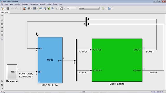
Let’s switch to Simulink to build the autonomous steering control system. This is the standard MPC control diagram that we want to build. We’ll start by adding the plant to our model. Here, I have a custom library, which includes the blocks I’ve previously created. The plant is one of them and has been developed as a state space model representing the lateral vehicle dynamics. The input to the plant is the steering angle, and the two outputs are the lateral position and the yaw angle. Now, we’re going to connect the MPC controller that you can find under Model Predictive Control Toolbox. The first input to this block is the measured outputs. So, we connect the outputs here. And the second input is the reference. In this example, we want to simulate a car changing lanes. To create a custom reference trajectory for such a scenario, I’m going to use the Driving Scenario Designer that is part of Automated Driving Toolbox. Using this app, I create a road with two lanes that are 4 meters wide, then add a car and add waypoints to generate the lane-change maneuver. You can adjust the waypoints manually from the side panel if needed. The car’s speed is set to 15 m/s. If I now simulate this scenario step by step, the app shows me how the yaw angle changes. I exported this scenario as a MATLAB function and created a block that outputs the reference lateral position and yaw angle values. I add this custom reference to my model and connect it to the controller. Here, we assume there are no measured disturbances, so we’ll remove the third input. Now that we connected all system components, we’ll continue designing the MPC controller. For this, we open the MPC block and click on “Design,” which opens up the MPC Designer. The MPC Designer is an interactive tool that lets you design MPC controllers and is shipped as part of Model Predictive Control Toolbox. Remember in the previous videos we talked about MPC design parameters such as sample time, prediction and control horizons, and constraints and weights. You can specify all these parameters in the MPC Designer, tune the controller, and then evaluate the controller’s performance. Now, we’ll go back to the MPC Designer and start by defining the MPC structure. We’ll enter the number of manipulated variables and measured outputs, and set the controller sample time to 0.1s. Then we click “define and linearize.” Remember that MPC uses an internal plant model to make predictions and an optimizer to find the optimal control action. Now, when we click “define and linearize,” the app imports and linearizes the plant from the Simulink model and uses it as the internal plant model. It also runs the default simulation scenario and displays the input and output responses. Next, we click on the I/O Attributes to type in the signal labels and units. Note that if these signals differ too much in magnitude, for example, say one is around 1 and the other one is around 1000, then you can use scale factors to bring them to similar scale. We’ll keep the default values for this example as the magnitude difference is not too much. Next, we’ll edit the default scenario. We can choose different types of reference signals from these options. The closest to our lane change scenario would be a ramp input for the lateral position reference and a constant reference of zero for the yaw angle to minimize it. We click OK and this updates the responses. Next, we’ll switch to the tuning tab where we can specify MPC design parameters. These are the default values for prediction and control horizons. Let’s see how the system behavior changes for a larger prediction horizon. For 15 and 20, the response looks more sluggish, so we will set it back to 10. Next, we’ll play with the control horizon. Increasing it to 3 provides a better control of the lateral position. If we increase it further, it doesn’t affect the response significantly, so we settle on a control horizon of 3.
Next, we’ll set the constraints. The input constraints are dictated by the physical limitations of the vehicle. In this example, we’ll assume that the steering can turn a maximum of 30 degrees, so we’ll input pi/6 radians for the input constraints. And for driver comfort, we’ll limit the rate of change of the steering angle to 15 degrees/sec. Note that all the input constraints are hard and the output constraints are soft by default. We’ll try to keep the outputs between these values. Next, we’ll specify the weights. If we want the inputs and outputs have a target, we need to set the weights to a nonzero value. For steering angle, we’ll keep the default weight of zero, as it doesn’t need to track a target. We’ll also keep the default weight for the input rate. You can increase this weight if you want to have even smaller input increments. And for the outputs, we’ll set the weight for the lateral position to 1 and the yaw angle weight to 0.1, as position tracking is our primary objective. After setting all these parameters, you can fine tune your controller by using this slider. We’ll slide it right for a more aggressive control. And the response looks good.
Now that we’re satisfied with the controller performance, we click on “export controller,” which updates the MPC controller block and runs the simulation. Note that in our Simulink model, we use the custom reference that we’ve designed before for the lane change scenario. Now we can look at the simulation results. We get satisfactory tracking for both outputs. And the steering angle is kept within the limits by the controller.
In this video, we’ve walked through the design process of an MPC controller but let me also mention that in Release 2018a there’s a Lane Keep Assist System block that effectively simplifies the design process. Check out the links in the video description to find out more on this.
We showed that the designed controller performs well, but note that the car dynamics we’ve used work for a specific operating condition, which is when we have a longitudinal speed of 15 m/s. If, however, the longitudinal speed of the car changes as it travels, the dynamics of the car will change, too. So, if we now change the speed to 35 m/s, this will cause the controller to degrade. In order to deal with this, we need to design an adaptive MPC controller that will update the internal plant model for changing operating conditions. And this is what we’re going to discuss in the next video.


