Main Content

SeriesNetwork

Series network for deep learning

Description

A series network is a neural network for deep learning with layers arranged one after the other. It has a single input layer and a single output layer.

Creation

There are several ways to create a SeriesNetwork object:

Note

To learn about other pretrained networks, such as googlenet and resnet50, see Pretrained Deep Neural Networks.

Properties

expand all

This property is read-only.

Network layers, specified as a Layer array.

This property is read-only.

Names of the input layers, specified as a cell array of character vectors.

Data Types: cell

This property is read-only.

Names of the output layers, specified as a cell array of character vectors.

Data Types: cell

Object Functions

activationsCompute deep learning network layer activations
classifyClassify data using trained deep learning neural network
predictPredict responses using trained deep learning neural network
predictAndUpdateStatePredict responses using a trained recurrent neural network and update the network state
classifyAndUpdateStateClassify data using a trained recurrent neural network and update the network state
resetStateReset state parameters of neural network
plotPlot neural network architecture

Examples

collapse all

Load a pretrained AlexNet convolutional neural network and examine the layers and classes.

Load the pretrained AlexNet network using alexnet. The output net is a SeriesNetwork object.

net = alexnet
net = 
  SeriesNetwork with properties:

    Layers: [25×1 nnet.cnn.layer.Layer]

Using the Layers property, view the network architecture. The network comprises of 25 layers. There are 8 layers with learnable weights: 5 convolutional layers, and 3 fully connected layers.

net.Layers
ans = 
  25x1 Layer array with layers:

     1   'data'     Image Input                   227x227x3 images with 'zerocenter' normalization
     2   'conv1'    Convolution                   96 11x11x3 convolutions with stride [4  4] and padding [0  0  0  0]
     3   'relu1'    ReLU                          ReLU
     4   'norm1'    Cross Channel Normalization   cross channel normalization with 5 channels per element
     5   'pool1'    Max Pooling                   3x3 max pooling with stride [2  2] and padding [0  0  0  0]
     6   'conv2'    Grouped Convolution           2 groups of 128 5x5x48 convolutions with stride [1  1] and padding [2  2  2  2]
     7   'relu2'    ReLU                          ReLU
     8   'norm2'    Cross Channel Normalization   cross channel normalization with 5 channels per element
     9   'pool2'    Max Pooling                   3x3 max pooling with stride [2  2] and padding [0  0  0  0]
    10   'conv3'    Convolution                   384 3x3x256 convolutions with stride [1  1] and padding [1  1  1  1]
    11   'relu3'    ReLU                          ReLU
    12   'conv4'    Grouped Convolution           2 groups of 192 3x3x192 convolutions with stride [1  1] and padding [1  1  1  1]
    13   'relu4'    ReLU                          ReLU
    14   'conv5'    Grouped Convolution           2 groups of 128 3x3x192 convolutions with stride [1  1] and padding [1  1  1  1]
    15   'relu5'    ReLU                          ReLU
    16   'pool5'    Max Pooling                   3x3 max pooling with stride [2  2] and padding [0  0  0  0]
    17   'fc6'      Fully Connected               4096 fully connected layer
    18   'relu6'    ReLU                          ReLU
    19   'drop6'    Dropout                       50% dropout
    20   'fc7'      Fully Connected               4096 fully connected layer
    21   'relu7'    ReLU                          ReLU
    22   'drop7'    Dropout                       50% dropout
    23   'fc8'      Fully Connected               1000 fully connected layer
    24   'prob'     Softmax                       softmax
    25   'output'   Classification Output         crossentropyex with 'tench' and 999 other classes

You can view the names of the classes learned by the network by viewing the Classes property of the classification output layer (the final layer). View the first 10 classes by selecting the first 10 elements.

net.Layers(end).Classes(1:10)
ans = 10×1 categorical array
     tench 
     goldfish 
     great white shark 
     tiger shark 
     hammerhead 
     electric ray 
     stingray 
     cock 
     hen 
     ostrich 

Specify the example file 'digitsnet.prototxt' to import.

protofile = 'digitsnet.prototxt';

Import the network layers.

layers = importCaffeLayers(protofile)
layers = 

  1x7 Layer array with layers:

     1   'testdata'   Image Input             28x28x1 images
     2   'conv1'      Convolution             20 5x5x1 convolutions with stride [1  1] and padding [0  0]
     3   'relu1'      ReLU                    ReLU
     4   'pool1'      Max Pooling             2x2 max pooling with stride [2  2] and padding [0  0]
     5   'ip1'        Fully Connected         10 fully connected layer
     6   'loss'       Softmax                 softmax
     7   'output'     Classification Output   crossentropyex with 'class1', 'class2', and 8 other classes

Load the data as an ImageDatastore object.

digitDatasetPath = fullfile(matlabroot,'toolbox','nnet', ...
    'nndemos','nndatasets','DigitDataset');
imds = imageDatastore(digitDatasetPath, ...
    'IncludeSubfolders',true, ...
    'LabelSource','foldernames');
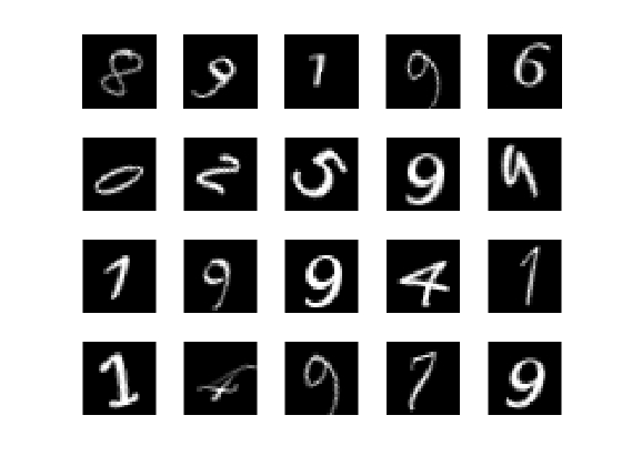
The datastore contains 10,000 synthetic images of digits from 0 to 9. The images are generated by applying random transformations to digit images created with different fonts. Each digit image is 28-by-28 pixels. The datastore contains an equal number of images per category.

Display some of the images in the datastore.

figure
numImages = 10000;
perm = randperm(numImages,20);
for i = 1:20
    subplot(4,5,i);
    imshow(imds.Files{perm(i)});
    drawnow;
end

Figure contains 20 axes objects. Axes object 1 contains an object of type image. Axes object 2 contains an object of type image. Axes object 3 contains an object of type image. Axes object 4 contains an object of type image. Axes object 5 contains an object of type image. Axes object 6 contains an object of type image. Axes object 7 contains an object of type image. Axes object 8 contains an object of type image. Axes object 9 contains an object of type image. Axes object 10 contains an object of type image. Axes object 11 contains an object of type image. Axes object 12 contains an object of type image. Axes object 13 contains an object of type image. Axes object 14 contains an object of type image. Axes object 15 contains an object of type image. Axes object 16 contains an object of type image. Axes object 17 contains an object of type image. Axes object 18 contains an object of type image. Axes object 19 contains an object of type image. Axes object 20 contains an object of type image.

Divide the datastore so that each category in the training set has 750 images and the testing set has the remaining images from each label.

numTrainingFiles = 750;
[imdsTrain,imdsTest] = splitEachLabel(imds,numTrainingFiles,'randomize');

splitEachLabel splits the image files in digitData into two new datastores, imdsTrain and imdsTest.

Define the convolutional neural network architecture.

layers = [ ...
    imageInputLayer([28 28 1])
    convolution2dLayer(5,20)
    reluLayer
    maxPooling2dLayer(2,'Stride',2)
    fullyConnectedLayer(10)
    softmaxLayer
    classificationLayer];
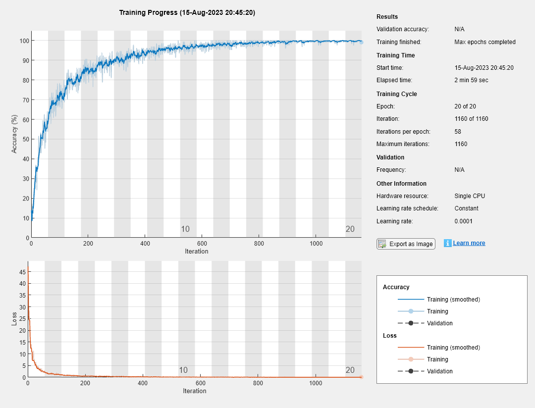
Set the options to the default settings for the stochastic gradient descent with momentum. Set the maximum number of epochs at 20, and start the training with an initial learning rate of 0.0001.

options = trainingOptions('sgdm', ...
    'MaxEpochs',20,...
    'InitialLearnRate',1e-4, ...
    'Verbose',false, ...
    'Plots','training-progress');

Train the network.

net = trainNetwork(imdsTrain,layers,options);

Figure Training Progress (19-Aug-2023 11:53:04) contains 2 axes objects and another object of type uigridlayout. Axes object 1 with xlabel Iteration, ylabel Loss contains 6 objects of type patch, text, line. Axes object 2 with xlabel Iteration, ylabel Accuracy (%) contains 6 objects of type patch, text, line.

Run the trained network on the test set, which was not used to train the network, and predict the image labels (digits).

YPred = classify(net,imdsTest);
YTest = imdsTest.Labels;

Calculate the accuracy. The accuracy is the ratio of the number of true labels in the test data matching the classifications from classify to the number of images in the test data.

accuracy = sum(YPred == YTest)/numel(YTest)
accuracy = 0.9400

Extended Capabilities

Version History

Introduced in R2016a