simsmooth

State-space model simulation smoother

Syntax

X = simsmooth(Mdl,Y)

X = simsmooth(Mdl,Y,Name=Value)

Description

X = simsmooth(Mdl,Y) returns simulated states X by applying a simulation smoother to the time-invariant or time-varying state-space model Mdl and responses Y. simsmooth uses forward filtering and back sampling to obtain one random path from the posterior distribution of the states.

X = simsmooth(Mdl,Y,Name=Value) returns simulated states with additional options specified by one or more name-value arguments. For example, simsmooth(Mdl,Y,NumPaths=100) returns 100 independently generated paths of states.

Examples

Simulate States of Time-Invariant State-Space Models Using Simulation Smoother

Suppose that a latent process is an AR(1) model. The state equation is

$$x_t=0.5x_{t-1}+u_t,$$

where $$u_t$$ is Gaussian with mean 0 and standard deviation 1.

Generate a random series of 100 observations from $$x_t$$, assuming that the series starts at 1.5.

T = 100;
ARMdl = arima('AR',0.5,'Constant',0,'Variance',1);
x0 = 1.5;
rng(1); % For reproducibility
x = simulate(ARMdl,T,'Y0',x0);

Suppose further that the latent process is subject to additive measurement error. The observation equation is

$$y_t=x_t+{\epsilon }_t,$$

where $${\epsilon }_t$$ is Gaussian with mean 0 and standard deviation 0.75. Together, the latent process and observation equations compose a state-space model.

Use the random latent state process (x) and the observation equation to generate observations.

y = x + 0.75*randn(T,1);

Specify the four coefficient matrices.

A = 0.5;
B = 1;
C = 1;
D = 0.75;

Specify the state-space model using the coefficient matrices.

Mdl = ssm(A,B,C,D)

Mdl = 
State-space model type: ssm

State vector length: 1
Observation vector length: 1
State disturbance vector length: 1
Observation innovation vector length: 1
Sample size supported by model: Unlimited

State variables: x1, x2,...
State disturbances: u1, u2,...
Observation series: y1, y2,...
Observation innovations: e1, e2,...

State equation:
x1(t) = (0.50)x1(t-1) + u1(t)

Observation equation:
y1(t) = x1(t) + (0.75)e1(t)

Initial state distribution:

Initial state means
 x1 
  0 

Initial state covariance matrix
     x1   
 x1  1.33 

State types
     x1     
 Stationary 

Mdl is an ssm model. Verify that the model is correctly specified using the display in the Command Window. The software infers that the state process is stationary. Subsequently, the software sets the initial state mean and covariance to the mean and variance of the stationary distribution of an AR(1) model.

Simulate one path each of states and observations. Specify that the paths span 100 periods.

simX = simsmooth(Mdl,y);

simX is a 100-by-1 vector of simulated states.

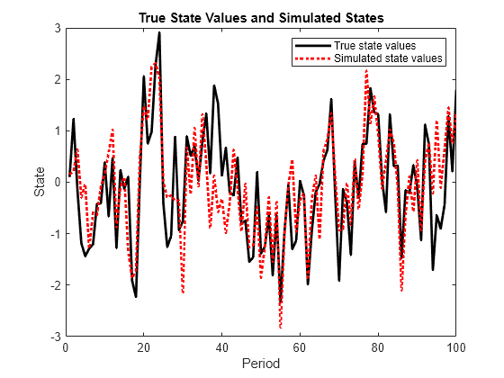
Plot the true state values with the simulated states.

figure;
plot(1:T,x,'-k',1:T,simX,':r','LineWidth',2);
title 'True State Values and Simulated States';
xlabel 'Period';
ylabel 'State';
legend({'True state values','Simulated state values'});

By default, simulate simulates one path for each state in the state-space model. To conduct a Monte Carlo study, specify to simulate a large number of paths using the 'NumPaths' name-value pair argument.

Estimate Posterior Distribution of States in State-Space Model

The simsmooth function draws random samples from the distribution of smoothed states, or the distribution of a state given all of the data and parameters. This is the definition of posterior distribution of a state. Suppose that a latent process is an AR(1). The state equation is

$$x_t=0.5x_{t-1}+u_t,$$

where $$u_t$$ is Gaussian with mean 0 and standard deviation 1.

Generate a random series of 100 observations from $$x_t$$, assuming that the series starts at 1.5.

T = 100;
ARMdl = arima('AR',0.5,'Constant',0,'Variance',1);
x0 = 1.5;
rng(1); % For reproducibility
x = simulate(ARMdl,T,'Y0',x0);

Suppose further that the latent process is subject to additive measurement error. The observation equation is

$$y_t=x_t+{\epsilon }_t,$$

where $${\epsilon }_t$$ is Gaussian with mean 0 and standard deviation 0.75. Together, the latent process and observation equations compose a state-space model.

Use the random latent state process (x) and the observation equation to generate observations.

y = x + 0.75*randn(T,1);

Specify the four coefficient matrices.

A = 0.5;
B = 1;
C = 1;
D = 0.75;

Specify the state-space model using the coefficient matrices.

Mdl = ssm(A,B,C,D);

Smooth the states of the state space model.

xsmooth = smooth(Mdl,y);

Draw 1000 paths from the posterior distribution of $$x_1$$.

N = 1000;
SimX = simsmooth(Mdl,y,'NumPaths',N);

SimX is a 100-by- 1-by- 1000 array. Rows correspond to periods, columns correspond to individual states, and leaves correspond to separate paths.

Because SimX has a singleton dimension, collapse it so that its leaves correspond to the columns using squeeze.

SimX = squeeze(SimX);

Compute the mean, standard deviation, and 95% confidence intervals of the state at each period.

xbar = mean(SimX,2);
xstd = std(SimX,[],2);
ci = [xbar - 1.96*xstd, xbar + 1.96*xstd];

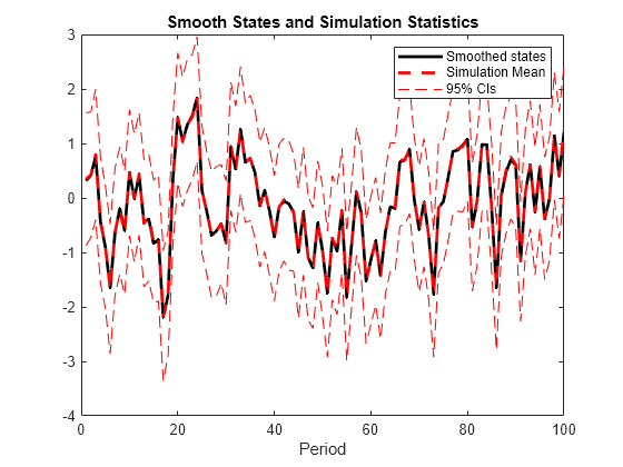
Plot the smoothed states, and the means and 95% confidence intervals of the draws at each period.

figure;
plot(xsmooth,'k','LineWidth',2);
hold on;
plot(xbar,'--r','LineWidth',2);
plot(1:T,ci(:,1),'--r',1:T,ci(:,2),'--r');
legend('Smoothed states','Simulation Mean','95% CIs');
title('Smooth States and Simulation Statistics');
xlabel('Period')

Input Arguments

Mdl — Standard state-space model

ssm model object

Standard state-space model, specified as anssm model object returned by ssm or estimate. A standard state-space model has finite initial state covariance matrix elements. That is, Mdl cannot be a dssm model object.

If Mdl is not fully specified (that is, Mdl contains unknown parameters), then specify values for the unknown parameters using the 'Params' Name,Value pair argument. Otherwise, the software throws an error.

Y — Observed response data

numeric matrix | cell vector of numeric vectors

Observed response data, specified as a numeric matrix or a cell vector of numeric vectors.

• If Mdl is time invariant with respect to the observation equation, then Y is a T-by-n matrix, where each row corresponds to a period and each column corresponds to a particular observation in the model. T is the sample size and m is the number of observations per period. The last row of Y contains the latest observations.

• If Mdl is time varying with respect to the observation equation, then Y is a T-by-1 cell vector. Each element of the cell vector corresponds to a period and contains an n_t-dimensional vector of observations for that period. The corresponding dimensions of the coefficient matrices in Mdl.C{t} and Mdl.D{t} must be consistent with the matrix in Y{t} for all periods. The last cell of Y contains the latest observations.

NaN elements indicate missing observations. For details on how the Kalman filter accommodates missing observations, see Algorithms.

Name-Value Arguments

Specify optional pairs of arguments as Name1=Value1,...,NameN=ValueN, where Name is the argument name and Value is the corresponding value. Name-value arguments must appear after other arguments, but the order of the pairs does not matter.

Before R2021a, use commas to separate each name and value, and enclose Name in quotes.

Example: simsmooth(Mdl,Y,NumPaths=100) returns 100 independently generated paths of states.

NumOut — Number of output arguments of parameter-to-matrix mapping function

positive integer

Number of output arguments of the parameter-to-matrix mapping function for implicitly defined state-space models, specified as the comma-separated pair consisting of 'NumOut' and a positive integer.

If you implicitly define a state-space model and you do not supply NumOut, then the software automatically detects the number of output arguments of the parameter-to-matrix mapping function. Such detection consumes extra resources, and might slow the simulation smoother.

For explicitly defined models, the software ignores NumOut and displays a warning message.

NumPaths — Number of sample paths to generate variants

1 (default) | positive integer

Number of sample paths to generate variants, specified as the comma-separated pair consisting of 'NumPaths' and a positive integer.

Example: 'NumPaths',1000

Data Types: double

Params — Values for unknown parameters

numeric vector

Values for unknown parameters in the state-space model, specified as the comma-separated pair consisting of 'Params' and a numeric vector.

The elements of Params correspond to the unknown parameters in the state-space model matrices A, B, C, and D, and, optionally, the initial state mean Mean0 and covariance matrix Cov0.

• If you created Mdl explicitly (that is, by specifying the matrices without a parameter-to-matrix mapping function), then the software maps the elements of Params to NaNs in the state-space model matrices and initial state values. The software searches for NaNs column-wise following the order A, B, C, D, Mean0, and Cov0.

• If you created Mdl implicitly (that is, by specifying the matrices with a parameter-to-matrix mapping function), then you must set initial parameter values for the state-space model matrices, initial state values, and state types within the parameter-to-matrix mapping function.

If Mdl contains unknown parameters, then you must specify their values. Otherwise, the software ignores the value of Params.

Data Types: double

Tolerance — Forecast uncertainty threshold

0 (default) | nonnegative scalar

Forecast uncertainty threshold, specified as the comma-separated pair consisting of 'Tolerance' and a nonnegative scalar.

If the forecast uncertainty for a particular observation is less than Tolerance during numerical estimation, then the software removes the uncertainty corresponding to the observation from the forecast covariance matrix before its inversion.

It is best practice to set Tolerance to a small number, for example, le-15, to overcome numerical obstacles during estimation.

Example: 'Tolerance',le-15

Data Types: double

Output Arguments

X — Simulated states

numeric matrix | cell matrix of numeric vectors

Simulated states, returned as a numeric matrix or cell matrix of vectors.

If Mdl is a time-invariant model with respect to the states, then X is a numObs-by-m-by-numPaths array. That is, each row corresponds to a period, each column corresponds to a state in the model, and each page corresponds to a sample path. The last row corresponds to the latest simulated states.

If Mdl is a time-varying model with respect to the states, then X is a numObs-by-numPaths cell matrix of vectors. X{t,j} contains a vector of length m_t of simulated states for period t of sample path j. The last row of X contains the latest set of simulated states.

More About

Simulation Smoother

The simulation smoother is an algorithm for drawing samples from the conditional, joint, posterior distribution of the states given the complete observed response series. You can use these random draws to conduct a simulation study of the estimators.

For a univariate, time-invariant state-space model, the simulation smoother algorithm follows these steps.

1. Obtain the smoothed states ($${\widehat{x}}_t;t=1,\mathrm{..},T$$) using the Kalman filter.

2. Choose initial state mean and variance values. Draw the initial random state $$x_0^{\ast }$$ from the Gaussian distribution with the initial state mean and variance.

3. Randomly generate T state disturbances and observation innovations from the standard normal distribution. Denote the random variants for period t $${\epsilon }_t^{\ast }$$ and $$u_t^{\ast }$$, respectively.

4. Create random observations and states by evaluating the state-space model

   $$\begin{array}{c}{x}_t^{\ast }=A{x}_{t-1}^{\ast }+B{\epsilon }_t^{\ast }\\ y_t^{\ast }=C{x}_t^{\ast }+D{u}_t^{\ast }\end{array}$$

   at $${\epsilon }_t^{\ast }$$ and $$u_t^{\ast }$$.

5. Obtain smoothed states ($${\widehat{x}}_t^{\ast }$$) by applying the Kalman filter to the state-space model using the observation series $$y_t^{\ast }$$.

6. Obtain the random path of smoothed states from the posterior distribution using

   $${\tilde{x}}_t={\widehat{x}}_t-{\widehat{x}}_t^{\ast }+x_t^{\ast }.$$

For more details, see [1].

Algorithms

• The Kalman filter accommodates missing data by not updating filtered state estimates corresponding to missing observations. In other words, suppose there is a missing observation at period t. Then, the state forecast for period t based on the previous t – 1 observations and filtered state for period t are equivalent.

• For increased speed in simulating states, the simulation smoother implements minimal dimensionality error checking. Therefore, for models with unknown parameter values, you should ensure that the dimensions of the data and the dimensions of the coefficient matrices are consistent.

References

[1] Durbin J., and S. J. Koopman. “A Simple and Efficient Simulation Smoother for State Space Time Series Analysis.” Biometrika. Vol 89., No. 3, 2002, pp. 603–615.

[2] Durbin, J, and Siem Jan Koopman. Time Series Analysis by State Space Methods. 2nd ed. Oxford: Oxford University Press, 2012.

Version History

Introduced in R2014b