Tune FIS Tree at the Command Line
This example shows how to tune membership function (MF) and rule parameters of a FIS tree. This example uses particle swarm and pattern search optimization, which require Global Optimization Toolbox software.
For more information on FIS trees, see FIS Trees.
For an example that interactively tunes a FIS tree using the same data, see Tune FIS Tree Using Fuzzy Logic Designer.
For an example that programmatically tunes a FIS using the same data, see Tune Fuzzy Inference System at the Command Line.
Load Example Data
This example trains a FIS using automobile fuel consumption data. The goal is for the FIS to predict fuel consumption in miles per gallon (MPG) using several automobile profile attributes. The training data is available in the University of California at Irvine Machine Learning Repository and contains data collected from automobiles of various makes and models.
This example uses the following six input data attributes to predict the output data attribute MPG with a FIS:
Number of cylinders
Displacement
Horsepower
Weight
Acceleration
Model year
Load the data. Each row of the data set obtained from the repository represents a different automobile profile.
[data,name] = loadGasData;
data contains 7 columns, where the first six columns contain the input attribute values. The final column contains the predicted MPG output. Split data into input and output data sets, X and Y, respectively.
X = data(:,1:6);
Y = data(:,7);
Partition the input and output data sets into training data (odd-indexed samples) and validation data (even-indexed samples).
trnX = X(1:2:end,:); % Training input data set
trnY = Y(1:2:end,:); % Training output data set
vldX = X(2:2:end,:); % Validation input data set
vldY = Y(2:2:end,:); % Validation output data set
Extract the range of each data attribute, which you will use for input/output range definition during FIS construction.
dataRange = [min(data)' max(data)'];
Construct FIS Tree
For this example, construct a FIS tree using the following steps:
Rank the input attributes based on their correlations with the output attribute.
Create multiple FIS objects using the ranked input attributes.
Construct a FIS tree from the FIS objects.
Rank Inputs According to Correlation Coefficients
Calculate the correlation coefficients for the training data. In the final row of the correlation matrix, the first six elements show the correlation coefficients between the six put data attributes and the output attribute.
c1 = corrcoef(data);
c1(end,:)
ans = 1×7

   -0.7776   -0.8051   -0.7784   -0.8322    0.4233    0.5805    1.0000
The first four input attributes have negative values, and the last two input attributes have positive values.
Rank the input attributes that have negative correlations in descending order by the absolute value of their correlation coefficients.
Weight
Displacement
Horsepower
Number of cylinders
Rank the input attributes that have positive correlations in descending order by the absolute value of their correlation coefficients.
Model year
Acceleration
These rankings show that the weight and model year have the highest negative and positive correlations with MPG, respectively.
Create Fuzzy Inference Systems
For this example, implement a FIS tree with the following structure.

The FIS tree uses multiple two-input-one-output FIS objects to reduce the total number of rules used In the inference process. fis1, fis2, and fis3 directly take the input values and generate intermediate MPG values, which are further combined using fis4 and fis5.
Input attributes with negative and positive correlation values are paired up to combine both positive and negative effects on the output for prediction. The inputs are grouped according to their ranks as follows:
Weight and model year
Displacement and acceleration
Horsepower and number of cylinders
The last group includes only inputs with negative correlation values since there are only two inputs with positive correlation values.
This example uses Sugeno-type FIS objects for faster evaluation during the tuning process as compared to Mamdani systems. Each FIS includes two inputs and one output, where each input contains two default triangular membership functions (MFs), and the output includes 4 default constant MFs. Specify the input and output ranges using the corresponding data attribute ranges.
The first FIS combines the weight and model year attributes.
fis1 = sugfis(Name="fis1");
fis1 = addInput(fis1,dataRange(4,:),NumMFs=2,Name="weight");
fis1 = addInput(fis1,dataRange(6,:),NumMFs=2,Name="year");
fis1 = addOutput(fis1,dataRange(7,:),NumMFs=4);
The second FIS combines the displacement and acceleration attributes.
fis2 = sugfis(Name="fis2");
fis2 = addInput(fis2,dataRange(2,:),NumMFs=2,Name="displacement");
fis2 = addInput(fis2,dataRange(5,:),NumMFs=2,Name="acceleration");
fis2 = addOutput(fis2,dataRange(7,:),NumMFs=4);
The third FIS combines the horsepower and number of cylinder attributes.
fis3 = sugfis(Name="fis3");
fis3 = addInput(fis3,dataRange(3,:),NumMFs=2,Name="horsepower");
fis3 = addInput(fis3,dataRange(1,:),NumMFs=2,Name="cylinders");
fis3 = addOutput(fis3,dataRange(7,:),NumMFs=4);
The fourth FIS combines the outputs of the first and second FIS.
fis4 = sugfis(Name="fis4");
fis4 = addInput(fis4,dataRange(7,:),NumMFs=2);
fis4 = addInput(fis4,dataRange(7,:),NumMFs=2);
fis4 = addOutput(fis4,dataRange(7,:),NumMFs=4);
The final FIS combines the outputs of third and fourth FIS and generates the estimated MPG. This FIS has the same input and output ranges as the fourth FIS.
fis5 = fis4;
fis5.Name = "fis5";
fis5.Outputs(1).Name = "mpg";
Create FIS Tree
Connect the fuzzy systems (fis1, fis2, fis3, fis4, and fis5) according to the FIS tree diagram.
fisTin = fistree([fis1 fis2 fis3 fis4 fis5],[ ...
    "fis1/output1" "fis4/input1"; ...
    "fis2/output1" "fis4/input2"; ...
    "fis3/output1" "fis5/input2"; ...
    "fis4/output1" "fis5/input1"])
fisTin =
  fistree with properties:

                       Name: "fistreemodel"
                        FIS: [1×5 sugfis]
                Connections: [4×2 string]
                     Inputs: [6×1 string]
                    Outputs: "fis5/mpg"
    DisableStructuralChecks: 0

	See 'getTunableSettings' method for parameter optimization.
Tune FIS Tree with Training Data
Tuning is performed in two steps.
Learn the rule base while keeping the input and output MF parameters constant.
Tune the parameters of the input/output MFs and rules.
The first step is less computationally expensive due to the small number of rule parameters, and it quickly converges to a fuzzy rule base during training. In the second step, using the rule base from the first step as an initial condition provides fast convergence of the parameter tuning process.
Learn Rules
To learn a rule base, first specify tuning options using a tunefisOptions object. Global optimization methods (genetic algorithm or particle swarm) are suitable for initial training when all the parameters of a fuzzy system are untuned. For this example, tune the FIS tree using the particle swarm optimization method ("particleswarm").
To learn new rules, set the OptimizationType to "learning". Restrict the maximum number of rules to 4. The number of tuned rules of each FIS can be less than this limit, since the tuning process removes duplicate rules.
options = tunefisOptions( ...
    Method="particleswarm",...
    OptimizationType="learning", ...
    NumMaxRules=4);
If you have Parallel Computing Toolbox™ software, you can improve the speed of the tuning process by setting options.UseParallel to true. If you do not have Parallel Computing Toolbox software, set options.UseParallel to false.
Set the maximum number of iterations to 50. To reduce training error in the rule learning process, you can increase the number of iterations. However, using too many iterations can overtune the FIS tree to the training data, increasing the validation errors.
options.MethodOptions.MaxIterations = 50;
Since particle swarm optimization uses random search, to obtain reproducible results, initialize the random number generator to its default configuration.
rng("default")Tune the FIS tree using the specified tuning data and options. Set the input order of the training data according to the FIS tree connections as follows: weight, year, displacement, acceleration, horsepower, and cylinders.
inputOrders1 = [4 6 2 5 3 1];
orderedTrnX1 = trnX(:,inputOrders1);
Learning rules with tunefis function takes approximately 4 minutes. For this example, enable tuning by setting runtunefis to true. To load pretrained results without running tunefis, you can set runtunefis to false.
runtunefis = false;
Parameter settings can be empty when learning new rules. For more information, see tunefis.
if runtunefis
    fisTout1 = tunefis(fisTin,[],orderedTrnX1,trnY,options); %#ok<UNRCH>
else
    tunedfis = load("tunedfistreempgprediction.mat");
    fisTout1 = tunedfis.fisTout1;
    rmseValue = calculateRMSE(fisTout1,orderedTrnX1,trnY);
    fprintf("Training RMSE = %.3f MPG\n",rmseValue);
end
Training RMSE = 3.399 MPG
The Best f(x) column shows the training root mean squared error (RMSE).
The learning process produces a set of new rules for the FIS tree.
fprintf("Total number of rules = %d\n",numel([fisTout1.FIS.Rules]));Total number of rules = 17
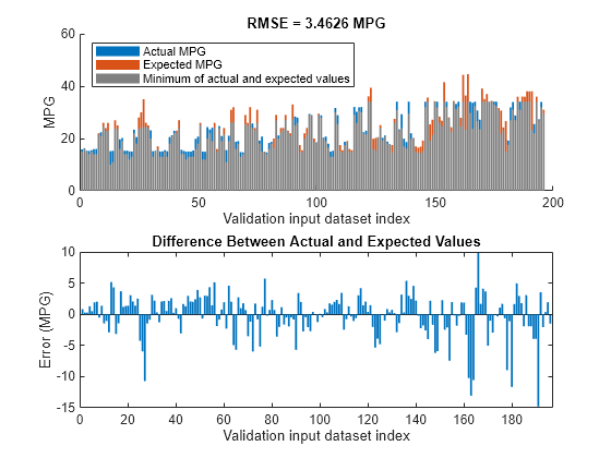
The learned system should have similar RMSE performance for both the training and validation data sets. To calculate the RMSE for the validation data set, evaluate fisout1 using validation input data set vldX. To hide run-time warnings during evaluation, set all the warning options to none.
Calculate the RMSE between the generated output data and the validation output data set vldY. Since the training and validation errors are similar, the learned system does not overfit the training data.
orderedVldX1 = vldX(:,inputOrders1);
plotActualAndExpectedResultsWithRMSE(fisTout1,orderedVldX1,vldY)

Tune All Parameters
After learning the new rules, tune the input/output MF parameters along with the parameters of the learned rules. To obtain the tunable parameters of the FIS tree, use the getTunableSettings function.
[in,out,rule] = getTunableSettings(fisTout1);
To tune the existing FIS tree parameter settings without learning new rules, set the OptimizationType to "tuning".
options.OptimizationType = "tuning";Since the FIS tree already learned rules using the training data, use a local optimization method for fast convergence of the parameter values. For this example, use the pattern search optimization method ("patternsearch").
options.Method = "patternsearch";Tuning the FIS tree parameters takes more iterations than the previous rule-learning step. Therefore, increase the maximum number of iterations of the tuning process to 75. As in the first tuning stage, you can reduce training errors by increasing the number of iterations. However, using too many iterations can overtune the parameters to the training data, increasing the validation errors.
options.MethodOptions.MaxIterations = 75;
To improve pattern search results, set method option UseCompletePoll to true.
options.MethodOptions.UseCompletePoll = true;
Tune the FIS tree parameters using the specified tunable settings, training data, and tuning options.
Tuning parameter values with tunefis function takes several minutes. To load pretrained results without running tunefis, you can set runtunefis to false.
rng("default")
if runtunefis
    fisTout2 = tunefis(fisTout1,[in;out;rule],orderedTrnX1,trnY,options); %#ok<UNRCH>
else
    fisTout2 = tunedfis.fisTout2;
    rmseValue = calculateRMSE(fisTout2,orderedTrnX1,trnY);
    fprintf("Training RMSE = %.3f MPG\n",rmseValue);
end
Training RMSE = 3.037 MPG
At the end of the tuning process, the training error reduces compared to the previous step.
Check Performance
Validate the performance of the tuned FIS tree, fisout2, using the validation input data set vldX.
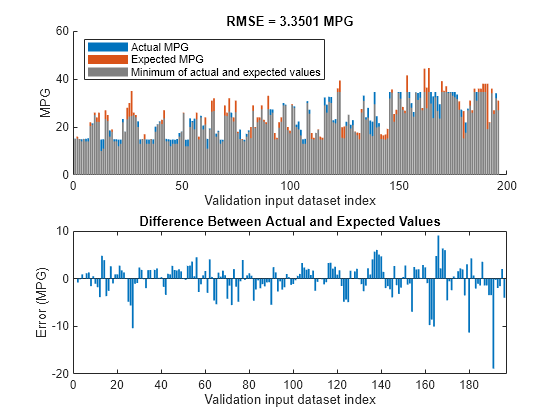
Compare the expected MPG obtained from the validation output data set vldY and actual MPG generated using fisout2. Compute the RMSE between these results.
plotActualAndExpectedResultsWithRMSE(fisTout2,orderedVldX1,vldY)

Tuning the FIS tree parameters improves the RMSE compared to the results from the initial learned rule base. Since the training and validation errors are similar, the parameters values are not overtuned.
Analyze Intermediate Data
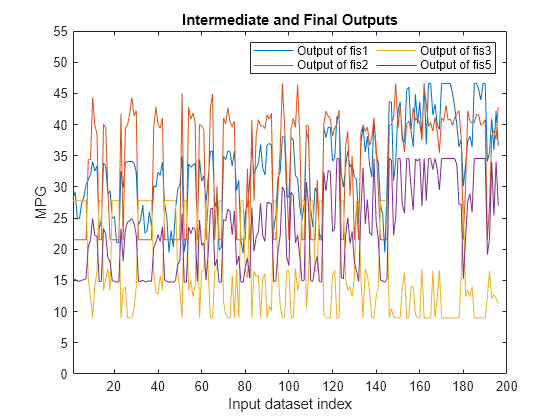
To gain insight into the operation of your system, you can add the outputs of the component fuzzy systems as outputs of your FIS tree. This is a benefit of using a FIS tree rather than a single monolithic FIS, as shown in Tune Fuzzy Inference System at the Command Line. Based on your analysis of the intermediate results, you can potentially improve the performance of your FIS tree.
For this example, to access the intermediate FIS outputs, add three additional outputs to the tuned FIS tree.
fisTout3 = fisTout2;
fisTout3.Outputs(end+1) = "fis1/output1";
fisTout3.Outputs(end+1) = "fis2/output1";
fisTout3.Outputs(end+1) = "fis3/output1";
To generate the additional outputs, evaluate the augmented FIS tree, fisTout3.
actY = evaluateFIS(fisTout3,orderedVldX1);
figure
plot(actY(:,[2 3 4 1]))
xlabel("Input dataset index")
ylabel("MPG")
axis([1 200 0 55])
legend(["Output of fis1" "Output of fis2" "Output of fis3" "Output of fis5"],...
    Location="NorthEast",NumColumns=2)
title("Intermediate and Final Outputs")

The final output of the FIS tree (fis5 output) appears to be highly correlated with the outputs of fis1 and fis3. To validate this assessment, check the correlation coefficients of the FIS outputs.
c2 = corrcoef(actY(:,[2 3 4 1]));
c2(end,:)
ans = 1×4

    0.9541    0.8245   -0.8427    1.0000
The last row of the correlation matrix shows that the outputs of fis1 and fis3 (first and third column, respectively) have higher correlations with the final output as compared to the output of fis2 (second column). This result indicates that simplifying the FIS tree by removing fis2 and fis4 and can potentially produce similar training results compared to the original tree structure.
Simplify and Retrain FIS Tree
Remove fis2 and fis4 from the FIS tree and connect the output of fis1 to the first input of fis5. When you remove a FIS from a FIS tree, any existing connections to that FIS are also removed.

fisTout3.FIS([2 4]) = [];
fisTout3.Connections(end+1,:) = ["fis1/output1" "fis5/input1"];
fis5.Inputs(1).Name = "fis1out";
To make the number of FIS tree outputs match the number of outputs in the training data, remove the FIS tree outputs from fis1 and fis3.
fisTout3.Outputs(2:end) = [];
Update the input training data order according to the new FIS tree input configuration.
inputOrders2 = [4 6 3 1];
orderedTrnX2 = trnX(:,inputOrders2);
Since the FIS tree configuration is changed, you must rerun both the learning and tuning steps. In the learning phase, the existing rule parameters are also tuned to fit the new configuration of the FIS tree.
options.Method = "particleswarm";
options.OptimizationType = "learning";
options.MethodOptions.MaxIterations = 50;

[~,~,rule] = getTunableSettings(fisTout3);

rng("default")
if runtunefis
    fisTout4 = tunefis(fisTout3,rule,orderedTrnX2,trnY,options); %#ok<UNRCH>
else
    fisTout4 = tunedfis.fisTout4;
    rmseValue = calculateRMSE(fisTout4,orderedTrnX2,trnY);
    fprintf("Training RMSE = %.3f MPG\n",rmseValue);
end
Training RMSE = 3.380 MPG
In the training phase, the parameters of the membership function and rules are tuned.
options.Method = "patternsearch";
options.OptimizationType = "tuning";
options.MethodOptions.MaxIterations = 75;
options.MethodOptions.UseCompletePoll = true;
[in,out,rule] = getTunableSettings(fisTout4);
rng("default")
if runtunefis
    fisTout5 = tunefis(fisTout4,[in;out;rule],orderedTrnX2,trnY,options); %#ok<UNRCH>
else
    fisTout5 = tunedfis.fisTout5;
    rmseValue = calculateRMSE(fisTout5,orderedTrnX2,trnY);
    fprintf("Training RMSE = %.3f MPG\n",rmseValue);
end
Training RMSE = 3.049 MPG
At the end of the tuning process, the FIS tree contains updated MF and rule parameter values. The rule base size of the new FIS tree configuration is smaller than the previous configuration.
fprintf("Total number of rules = %d\n",numel([fisTout5.FIS.Rules]));Total number of rules = 11
Check Performance of the Simplified FIS Tree
Evaluate the updated FIS tree using the four input attributes of the checking data set.
orderedVldX2 = vldX(:,inputOrders2);
plotActualAndExpectedResultsWithRMSE(fisTout5,orderedVldX2,vldY)

The simplified FIS tree with four input attributes produces better results in terms of RMSE as compared to the first configuration, which uses six input attributes. Therefore, it shows that a FIS tree can be represented with fewer number of inputs and rules to generalize the training data.
Conclusion
You can further improve the training error of the tuned FIS tree by:
Increasing number of iterations in both the rule-learning and parameter-tuning phases. Doing so increases the duration of the optimization process and can also increase validation error due to overtuned system parameters with the training data.
Using global optimization methods, such as
gaandparticleswarm, in both rule-learning and parameter-tuning phases.gaandparticleswarmperform better for large parameter tuning ranges since they are global optimizers. On the other hand,patternsearchandsimulannealbndperform better for small parameter ranges since they are local optimizers. If rules are already added to a FIS tree using training data, thenpatternsearchandsimulannealbndmay produce faster convergence as compared togaandparticleswarm. For more information on these optimization methods and their options, seega(Global Optimization Toolbox),particleswarm(Global Optimization Toolbox),patternsearch(Global Optimization Toolbox), andsimulannealbnd(Global Optimization Toolbox).Changing the FIS properties, such as the type of FIS, number of inputs, number of input/output MFs, MF types, and number of rules. For fuzzy systems with a large number of inputs, a Sugeno FIS generally converges faster than a Mamdani FIS since a Sugeno system has fewer output MF parameters (if
constantMFs are used) and faster defuzzification. Small numbers of MFs and rules reduce the number of parameters to tune, producing a faster tuning process. Furthermore, a large number of rules may overfit the training data.Modifying tunable parameter settings for MFs and rules. For example, you can tune the support of a triangular MF without changing its peak location. Doing so reduces the number of tunable parameters and can produce a faster tuning process for specific applications. For rules, you can exclude zero MF indices by setting the
AllowEmptytunable setting tofalse, which reduces the overall number of rules during the learning phase.Changing FIS tree properties, such as number of fuzzy systems and connections between the fuzzy systems.
Using different ranking and grouping of the inputs to the FIS tree.
Local Functions
function plotActualAndExpectedResultsWithRMSE(fis,x,y)

% Calculate RMSE between actual and expected results.
[rmse,actY] = calculateRMSE(fis,x,y);

% Plot results.
figure
subplot(2,1,1)
hold on
bar(actY)
bar(y)
bar(min(actY,y),FaceColor=[0.5 0.5 0.5])
hold off
axis([0 200 0 60])
xlabel("Validation input dataset index")
ylabel("MPG")
legend(["Actual MPG" "Expected MPG" "Minimum of actual and expected values"],...
    Location="NorthWest")
title("RMSE = " + num2str(rmse) + " MPG")

subplot(2,1,2)
bar(actY-y)
xlabel("Validation input dataset index")
ylabel("Error (MPG)")
title("Difference Between Actual and Expected Values")

end

function [rmse,actY] = calculateRMSE(fis,x,y)

% Evaluate FIS.
actY = evaluateFIS(fis,x);

% Calculate RMSE.
del = actY - y;
rmse = sqrt(mean(del.^2));

end

function y = evaluateFIS(fis,x)

% Specify options for FIS evaluation.
persistent evalOptions
if isempty(evalOptions)
    evalOptions = evalfisOptions( ...
        EmptyOutputFuzzySetMessage="none", ...
        NoRuleFiredMessage="none", ...
        OutOfRangeInputValueMessage="none");
end

% Evaluate FIS
y = evalfis(fis,x,evalOptions);

end
See Also
tunefis | sugfis | getTunableSettings | fistree