MapAxes Properties
MapAxes properties control the appearance and behavior of a
MapAxes object. By changing property values, you can modify certain aspects
of the map axes. Use dot notation to query and set properties.
p = projcrs(26919);
newmap(p)
mx = gca;
c = mx.OutlineColor;
mx.OutlineColor = "blue";
Map
Font
Text color for the title, the tick labels, and the scale bar, specified as an RGB triplet, a hexadecimal color code, a color name, or a short name.
For a custom color, specify an RGB triplet or a hexadecimal color code.
An RGB triplet is a three-element row vector whose elements specify the intensities of the red, green, and blue components of the color. The intensities must be in the range
[0,1], for example,[0.4 0.6 0.7].A hexadecimal color code is a string scalar or character vector that starts with a hash symbol (
#) followed by three or six hexadecimal digits, which can range from0toF. The values are not case sensitive. Therefore, the color codes"#FF8800","#ff8800","#F80", and"#f80"are equivalent.
Alternatively, you can specify some common colors by name. This table lists the named color options, the equivalent RGB triplets, and the hexadecimal color codes.
| Color Name | Short Name | RGB Triplet | Hexadecimal Color Code | Appearance |
|---|---|---|---|---|
"red" | "r" | [1 0 0] | "#FF0000" |
|
"green" | "g" | [0 1 0] | "#00FF00" |
|
"blue" | "b" | [0 0 1] | "#0000FF" |
|
"cyan"
| "c" | [0 1 1] | "#00FFFF" |
|
"magenta" | "m" | [1 0 1] | "#FF00FF" |
|
"yellow" | "y" | [1 1 0] | "#FFFF00" |
|
"black" | "k" | [0 0 0] | "#000000" |
|
"white" | "w" | [1 1 1] | "#FFFFFF" |
|
"none" | Not applicable | Not applicable | Not applicable | No color |
This table lists the default color palettes for plots in the light and dark themes.
| Palette | Palette Colors |
|---|---|
Before R2025a: Most plots use these colors by default. |
|
|
|
You can get the RGB triplets and hexadecimal color codes for these palettes using the orderedcolors and rgb2hex functions. For example, get the RGB triplets for the "gem" palette and convert them to hexadecimal color codes.
RGB = orderedcolors("gem");
H = rgb2hex(RGB);
Before R2023b: Get the RGB triplets using RGB =
get(groot,"FactoryAxesColorOrder").
Before R2024a: Get the hexadecimal color codes using H =
compose("#%02X%02X%02X",round(RGB*255)).
To use a different text color for the title than for the tick labels and scale bar,
set the Color property of the title, such as
mx.Title.Color = "blue".
To use a different text color for the scale bar than for the title and tick labels,
set the FontColor property of the scale bar, such as
mx.Scalebar.FontColor = "blue".
Example: mx.FontColor = [0 0 1];
Example: mx.FontColor = "b";
Example: mx.FontColor = "blue";
Example: mx.FontColor = "#0000FF";
Font name, specified as a supported font name or "FixedWidth". To
display and print text properly, you must choose a font that your system supports. The
default font depends on your operating system and locale.
To use a fixed-width font that looks good in any locale, specify
"FixedWidth". The fixed-width font relies on the root FixedWidthFontName
property. Setting the root FixedWidthFontName property causes the
display to immediately update to use the new font.
Font size, specified as a numeric scalar. The font size affects the title, tick labels, and
scale bar, as well as any legends or color bars associated with the axes. The default
font size depends on the specific operating system and locale. By default, the axes
object measures the font size in points. To change the units, set the
FontUnits property.
MATLAB automatically scales some of the text to a percentage of the axes font size.
Titles — 110% of the axes font size by default. To control title scaling, use the
TitleFontSizeMultiplierandLabelFontSizeMultiplierproperties.Legends and color bars — 90% of the axes font size by default. To specify a different font size, set the
FontSizeproperty for theLegendorColorBarobject instead.Scale bar — 80% of the axes font size by default. To specify a different font size, set the
FontSizeproperty for theGeographicScalebarobject instead.
Selection mode for the font size, specified as one of these values:
'auto'— Font size specified by MATLAB. If you resize the axes to be smaller than the default size, the font size might scale down to improve readability and layout.'manual'— Font size specified manually. Do not scale the font size as the axes size changes. To specify the font size, set theFontSizeproperty.
Character thickness, specified as "normal" or
"bold".
MATLAB uses the FontWeight property to select a font from
those available on your system. Not all fonts have a bold weight. Therefore, specifying
a bold font weight can still result in the normal font weight.
Character slant, specified as "normal" or
"italic".
Not all fonts have both font styles. Therefore, the italic font might look the same as the normal font.
Scale factor for the title font size, specified as a numeric value greater than 0. The scale factor is applied to the value of the FontSize property to determine the font size for the title.
Subtitle character thickness, specified as one of these values:
'normal'— Default weight as defined by the particular font'bold'— Thicker characters than normal
Ticks
Graticule
Color of the graticule lines, specified as an RGB triplet, a hexadecimal color code, a color name, or a short name.
For a custom color, specify an RGB triplet or a hexadecimal color code.
An RGB triplet is a three-element row vector whose elements specify the intensities of the red, green, and blue components of the color. The intensities must be in the range
[0,1], for example,[0.4 0.6 0.7].A hexadecimal color code is a string scalar or character vector that starts with a hash symbol (
#) followed by three or six hexadecimal digits, which can range from0toF. The values are not case sensitive. Therefore, the color codes"#FF8800","#ff8800","#F80", and"#f80"are equivalent.
Alternatively, you can specify some common colors by name. This table lists the named color options, the equivalent RGB triplets, and the hexadecimal color codes.
| Color Name | Short Name | RGB Triplet | Hexadecimal Color Code | Appearance |
|---|---|---|---|---|
"red" | "r" | [1 0 0] | "#FF0000" |
|
"green" | "g" | [0 1 0] | "#00FF00" |
|
"blue" | "b" | [0 0 1] | "#0000FF" |
|
"cyan"
| "c" | [0 1 1] | "#00FFFF" |
|
"magenta" | "m" | [1 0 1] | "#FF00FF" |
|
"yellow" | "y" | [1 1 0] | "#FFFF00" |
|
"black" | "k" | [0 0 0] | "#000000" |
|
"white" | "w" | [1 1 1] | "#FFFFFF" |
|
"none" | Not applicable | Not applicable | Not applicable | No color |
This table lists the default color palettes for plots in the light and dark themes.
| Palette | Palette Colors |
|---|---|
Before R2025a: Most plots use these colors by default. |
|
|
|
You can get the RGB triplets and hexadecimal color codes for these palettes using the orderedcolors and rgb2hex functions. For example, get the RGB triplets for the "gem" palette and convert them to hexadecimal color codes.
RGB = orderedcolors("gem");
H = rgb2hex(RGB);
Before R2023b: Get the RGB triplets using RGB =
get(groot,"FactoryAxesColorOrder").
Before R2024a: Get the hexadecimal color codes using H =
compose("#%02X%02X%02X",round(RGB*255)).
To set the outline color of the axes, use the OutlineColor
property.
Line style for graticule lines, specified as one of the line styles in this table.
| Line Style | Description | Resulting Line |
|---|---|---|
"-" | Solid line |
|
"--" | Dashed line |
|
":" | Dotted line |
|
"-." | Dash-dotted line |
|
"none" | No line | No line |
Width of the graticule lines, specified as a positive scalar in point units. One point equals 1/72 of an inch.
When the GraticuleLineWidthMode property has a value of
"auto", the value of GraticuleLineWidth
matches the value of LineWidth.
Selection mode for the GraticuleLineWidth property, specified
as one of these values:
"auto"— Automatically select the width of graticule lines based on the value of theLineWidthproperty."manual"— Manually specify the width of graticule lines. To specify the value, set theGraticuleLineWidthproperty.
Transparency of the graticule lines, specified as a value in the range [0, 1]. A
value of 1 means opaque and a value of 0 means
completely transparent.
Labels
Multiple Plots
| Palette | Palette Colors |
|---|---|
Before R2025a: Most plots use these colors by default. |
|
|
|
You can get the RGB triplets and hexadecimal color codes for these palettes using the orderedcolors and rgb2hex functions. For example, get the RGB triplets for the "gem" palette and convert them to hexadecimal color codes.
RGB = orderedcolors("gem");
H = rgb2hex(RGB);
Before R2023b: Get the RGB triplets using RGB =
get(groot,"FactoryAxesColorOrder").
Before R2024a: Get the hexadecimal color codes using H =
compose("#%02X%02X%02X",round(RGB*255)).
MATLAB assigns colors to objects according to their order of creation. For example, when plotting lines, the first line uses the first color, the second line uses the second color, and so on. If there are more lines than colors, then the cycle repeats.
Changing the Color Order Before or After Plotting
You can change the color order in either of these ways:
Call the
colororderfunction to change the color order for all the axes in a figure. The colors of existing plots in the figure update immediately. If you place additional axes into the figure, those axes also use the new color order. If you continue to call plotting commands, those commands also use the new colors.Set the
ColorOrderproperty on the axes, call theholdfunction to set the axes hold state to"on", and then call the desired plotting functions. Unlike thecolororderfunction, this process sets the color order for the specific axes rather than the entire figure. You must set theholdstate to"on"to ensure that subsequent plotting commands do not reset the axes to use the default color order.
Since R2023a
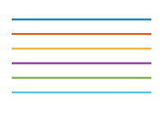
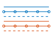
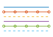
How to cycle through the line styles when there are multiple lines in the axes, specified as one of the values from this table.
The examples in this table were created using the default colors in the
ColorOrder property and three line styles
(["-","-o","--"]) in the LineStyleOrder
property.
| Value | Description | Example |
|---|---|---|
| Cycle through the line styles of the |
|
"beforecolor" | Cycle through the line styles of the
|
|
"withcolor" | Cycle through the line styles of the
|
|
This property is read-only.
SeriesIndex value for the next plot object added to the axes,
returned as a whole number greater than or equal to 0. This property
is useful when you want to track how the objects cycle through the colors and line
styles. This property maintains a count of the objects in the axes that have a numeric
SeriesIndex property value. MATLAB uses it to assign a SeriesIndex value to each new
object. The count starts at 1 when you create the axes, and it
increases by 1 for each additional object. Thus, the count is
typically n+1, where n is the number of objects in
the axes.
If you manually change the ColorOrderIndex or
LineStyleOrderIndex property on the axes, the value of the
NextSeriesIndex property changes to 0. As a
consequence, objects that have a SeriesIndex property no longer
update automatically when you change the ColorOrder or
LineStyleOrder properties on the axes.
Properties to reset when adding a new plot to the axes, specified as one of these values:
"add"— Add new plots to the existing axes. Do not delete existing plots or reset axes properties before displaying the new plot."replacechildren"— Delete existing plots before displaying the new plot. Reset theColorOrderIndexandLineStyleOrderIndexproperties to1, but do not reset other axes properties. The next plot added to the axes uses the first color and line style based on theColorOrderandLineStyleOrderproperties. This value is similar to usingclabefore every new plot."replace"— Delete existing plots and reset axes properties, exceptProjectedCRS,Position, andUnits, to their default values before displaying the new plot."replaceall"— Delete existing plots and reset axes properties, exceptPositionandUnits, to their default values before displaying the new plot. This value is similar to usingcla resetbefore every new plot.
Figures also have a NextPlot property.
Alternatively, you can use the newmap
function to prepare figures and axes for subsequent graphics commands.
Color order index, specified as a positive integer. This property specifies the next
color MATLAB selects from the axes ColorOrder property when it creates
the next plot object, such as a Line or Scatter
object. For example, if the color order index value is 1, then the
next object added to the axes uses the first color in the
ColorOrder matrix. If the index value exceeds the number of
colors in the ColorOrder matrix, then the index value modulo of the
number of colors in the ColorOrder matrix determines the color of
the next object.
When the NextPlot property of the axes is set to
'add', then the color order index value increases every time you
add a new plot to the axes. To start again with first color, set the
ColorOrderIndex property to 1.
Line style order index, specified as a positive integer. This property specifies the
next line style MATLAB selects from the axes LineStyleOrder property to
create the next plot line. For example, if this property is set to 1,
then the next plot line you add to the axes uses the first item in the
LineStyleOrder property. If the index value exceeds the number of
line styles in the LineStyleOrder array, then the index value
modulo of the number of elements in the LineStyleOrder array
determines the style of the next line.
When the NextPlot property of the axes is set to
"add", MATLAB increments the index value after cycling through all the colors in the
ColorOrder property with the current
line style. To start again with first line style, set the
LineStyleOrderIndex property to 1.
Color and Transparency Maps
Map Styling
Background color, specified as an RGB triplet, a hexadecimal color code, a color name, or a short name.
For a custom color, specify an RGB triplet or a hexadecimal color code.
An RGB triplet is a three-element row vector whose elements specify the intensities of the red, green, and blue components of the color. The intensities must be in the range
[0,1], for example,[0.4 0.6 0.7].A hexadecimal color code is a string scalar or character vector that starts with a hash symbol (
#) followed by three or six hexadecimal digits, which can range from0toF. The values are not case sensitive. Therefore, the color codes"#FF8800","#ff8800","#F80", and"#f80"are equivalent.
Alternatively, you can specify some common colors by name. This table lists the named color options, the equivalent RGB triplets, and the hexadecimal color codes.
| Color Name | Short Name | RGB Triplet | Hexadecimal Color Code | Appearance |
|---|---|---|---|---|
"red" | "r" | [1 0 0] | "#FF0000" |
|
"green" | "g" | [0 1 0] | "#00FF00" |
|
"blue" | "b" | [0 0 1] | "#0000FF" |
|
"cyan"
| "c" | [0 1 1] | "#00FFFF" |
|
"magenta" | "m" | [1 0 1] | "#FF00FF" |
|
"yellow" | "y" | [1 1 0] | "#FFFF00" |
|
"black" | "k" | [0 0 0] | "#000000" |
|
"white" | "w" | [1 1 1] | "#FFFFFF" |
|
"none" | Not applicable | Not applicable | Not applicable | No color |
This table lists the default color palettes for plots in the light and dark themes.
| Palette | Palette Colors |
|---|---|
Before R2025a: Most plots use these colors by default. |
|
|
|
You can get the RGB triplets and hexadecimal color codes for these palettes using the orderedcolors and rgb2hex functions. For example, get the RGB triplets for the "gem" palette and convert them to hexadecimal color codes.
RGB = orderedcolors("gem");
H = rgb2hex(RGB);
Before R2023b: Get the RGB triplets using RGB =
get(groot,"FactoryAxesColorOrder").
Before R2024a: Get the hexadecimal color codes using H =
compose("#%02X%02X%02X",round(RGB*255)).
Example: mx.Color = [0 0 1];
Example: mx.Color = "b";
Example: mx.Color = "blue";
Example: mx.Color = "#0000FF";
Color of the map outline, the ticks, and the edge of the scale bar, specified as an RGB triplet, a hexadecimal color code, a color name, or a short name.
For a custom color, specify an RGB triplet or a hexadecimal color code.
An RGB triplet is a three-element row vector whose elements specify the intensities of the red, green, and blue components of the color. The intensities must be in the range
[0,1], for example,[0.4 0.6 0.7].A hexadecimal color code is a string scalar or character vector that starts with a hash symbol (
#) followed by three or six hexadecimal digits, which can range from0toF. The values are not case sensitive. Therefore, the color codes"#FF8800","#ff8800","#F80", and"#f80"are equivalent.
Alternatively, you can specify some common colors by name. This table lists the named color options, the equivalent RGB triplets, and the hexadecimal color codes.
| Color Name | Short Name | RGB Triplet | Hexadecimal Color Code | Appearance |
|---|---|---|---|---|
"red" | "r" | [1 0 0] | "#FF0000" |
|
"green" | "g" | [0 1 0] | "#00FF00" |
|
"blue" | "b" | [0 0 1] | "#0000FF" |
|
"cyan"
| "c" | [0 1 1] | "#00FFFF" |
|
"magenta" | "m" | [1 0 1] | "#FF00FF" |
|
"yellow" | "y" | [1 1 0] | "#FFFF00" |
|
"black" | "k" | [0 0 0] | "#000000" |
|
"white" | "w" | [1 1 1] | "#FFFFFF" |
|
"none" | Not applicable | Not applicable | Not applicable | No color |
This table lists the default color palettes for plots in the light and dark themes.
| Palette | Palette Colors |
|---|---|
Before R2025a: Most plots use these colors by default. |
|
|
|
You can get the RGB triplets and hexadecimal color codes for these palettes using the orderedcolors and rgb2hex functions. For example, get the RGB triplets for the "gem" palette and convert them to hexadecimal color codes.
RGB = orderedcolors("gem");
H = rgb2hex(RGB);
Before R2023b: Get the RGB triplets using RGB =
get(groot,"FactoryAxesColorOrder").
Before R2024a: Get the hexadecimal color codes using H =
compose("#%02X%02X%02X",round(RGB*255)).
To use a different color for the edge of the scale bar than for the map outline and
ticks, set the EdgeColor property of the scale bar, such as
mx.Scalebar.EdgeColor = "blue".
Example: mx.OutlineColor = [0 0 1];
Example: mx.OutlineColor = "b";
Example: mx.OutlineColor = "blue";
Example: mx.OutlineColor = "#0000FF";
Line width of the axes outline, the tick marks, the graticule lines, and the edge of the scale bar, specified as a positive scalar in point units. One point equals 1/72 inch.
You can use a different line width for the graticule lines than for the axes outline
and tick marks by setting the GraticuleLineWidth property. The
LineWidth property controls the width of the graticule lines only
when the value of the GraticuleLineWidthMode property is
"auto".
To use a different line width for the edge of the scale bar than for the axes
outline, the tick marks, and the graticule lines, set the LineWidth
property of the scale bar, such as mx.Scalebar.LineWidth = 2.
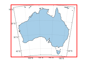
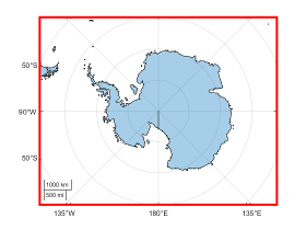
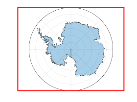
Map layout, specified as one of these options:
"normal"— Display data within the box specified byPosition. For many projected CRSs, this box includes the quadrangle defined byCartographicLatitudeLimitsandCartographicLongitudeLimitsand some areas surrounding the quadrangle. The axes does not display data where the projection has undefined numeric results or extreme map distortion."cartographic"— Display only the data within the quadrangle defined by theCartographicLatitudeLimitsandCartographicLongitudeLimitsproperties.
The "normal" option is appropriate for most data visualization
and exploration workflows. The "cartographic" option is useful when
creating static maps or when preparing maps for publication. For more information about
creating maps using the "cartographic" option, see Create Map of Quadrangle Using Cartographic Map Layout.
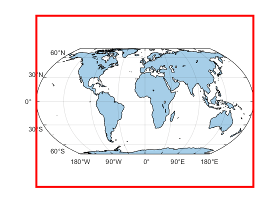
This table compares the "normal" and
"cartographic" options for several projected CRSs. The figures
within the table show the box specified by Position in red.
| Projected CRS | "normal" | "cartographic" |
|---|---|---|
A projected CRS for a temperate region. This row shows
maps created from a |
|
|
A projected CRS for a polar region. This row shows maps
created from a |
|
|
A projected CRS for a global region. This row shows
maps created from a In this case, the map layouts
for the |
|
|


Latitude limits for the quadrangle used by MapLayout, specified
as a two-element vector of the form [latmin latmax], where
latmax is greater than latmin.
By default, MATLAB sets this property using the area of use for
the projected CRS. When a projected CRS does not indicate the area of use, MATLAB sets this property to [-90 90].
Changing the value of this property does not change the value of
ProjectedCRS.
Panning or zooming within the map does not change the value of this property.
To change the geographic limits of a map that is in the default layout
(MapLayout is "normal"), use the geolimits
function instead of the CartographicLatitudeLimits and
CartographicLongitudeLimits properties.
Longitude limits for the quadrangle used by MapLayout,
specified as a two-element vector of the form [lonmin lonmax]. In
most cases, lonmax is greater than lonmin.
By default, MATLAB sets this property using the area of use for
the projected CRS. When a projected CRS does not indicate the area of use, MATLAB sets this property to [-180 180].
Changing the value of this property does not change the value of
ProjectedCRS.
Panning or zooming within the map does not change the value of this property.
To change the geographic limits of a map that is in the default layout
(MapLayout is "normal"), use the geolimits
function instead of the CartographicLatitudeLimits and
CartographicLongitudeLimits properties.
Position
Size and location, including the labels and a margin, specified as a four-element vector of the form [left bottom width height]. By default, MATLAB measures the values in units normalized to the container. To change the units, set the Units property. The default value of [0 0 1 1] includes the whole interior of the container.
The
leftandbottomelements define the distance from the lower-left corner of the container (typically a figure, panel, or tab) to the lower-left corner of the outer position boundary.The
widthandheightelements are the outer position boundary dimensions.
This figure shows the areas defined by the OuterPosition values (blue) and the Position values (red).

Note
Setting this property has no effect when the parent container is a
TiledChartLayout object.
Inner size and location, specified as a four-element vector of the form
[left bottom width height]. This property is equivalent to the
Position property.
Note
Setting this property has no effect when the parent container is a
TiledChartLayout object.
Size and location, excluding a margin for the labels, specified as a four-element vector of the form [left bottom width height]. By default, MATLAB measures the values in units normalized to the container. To change the units, set the Units property.
The
leftandbottomelements define the distance from the lower-left corner of the container (typically a figure, panel, or tab) to the lower-left corner of the position boundary.The
widthandheightelements are the position boundary dimensions.
If you want to specify the position and account for the text around the axes, then set the
OuterPosition property instead. This figure shows the areas
defined by the OuterPosition values (blue) and the
Position values (red).
Note
Setting this property has no effect when the parent container is a
TiledChartLayout object.
Position property to hold constant when adding, removing, or changing decorations, specified as one of the following values:
"outerposition"— TheOuterPositionproperty remains constant when you add, remove, or change decorations such as a title or an axis label. If any positional adjustments are needed, MATLAB adjusts theInnerPositionproperty."innerposition"— TheInnerPositionproperty remains constant when you add, remove, or change decorations such as a title or an axis label. If any positional adjustments are needed, MATLAB adjusts theOuterPositionproperty.
Note
Setting this property has no effect when the parent container is a
TiledChartLayout object.
Position units, specified as one of these values.
Units | Description |
|---|---|
"normalized" (default) | Normalized with respect to the container, which is typically the figure or a panel. The
lower-left corner of the container maps to (0,0)
and the upper-right corner maps to (1,1). |
"inches" | Inches. |
"centimeters" | Centimeters. |
"characters" | Based on the default
|
"points" | Typography points. One point equals 1/72 of an inch. |
"pixels" | Pixels. On Windows and Macintosh systems, the size of a pixel is 1/96th of an inch. This size is independent of your system resolution. On Linux systems, the size of a pixel is determined by your system resolution. |
When specifying the units using a name-value argument during object creation, you must set the
Units property before specifying the properties that you want
to use these units, such as Position.
Layout options, specified as a TiledChartLayoutOptions or a
GridLayoutOptions object. This property is useful when the axes
object is either in a tiled chart layout or a grid layout.
To position the axes within the grid of a tiled chart layout, set the
Tile and TileSpan properties on the
TiledChartLayoutOptions object. For example, consider a 3-by-3
tiled chart layout. The layout has a grid of tiles in the center, and four tiles along
the outer edges. In practice, the grid is invisible and the outer tiles do not take up
space until you populate them with axes or charts.

This code places the axes ax in the third tile of the
grid.
ax.Layout.Tile = 3;
To make the axes span multiple tiles, specify the TileSpan property as a two-element vector. For example, this axes spans 2 rows and 3 columns of tiles.
ax.Layout.TileSpan = [2 3];
To place the axes in one of the surrounding tiles, specify the
Tile property as 'north',
'south', 'east', or 'west'.
For example, setting the value to 'east' places the axes in the tile
to the right of the
grid.
ax.Layout.Tile = 'east';To place the axes into a layout within an app, specify this property as a
GridLayoutOptions object. For more information about working with
grid layouts in apps, see uigridlayout.
If the axes is not a child of either a tiled chart layout or a grid layout (for example, if it is a child of a figure or panel) then this property is empty and has no effect.
Interactivity
Since R2024a
Options to customize interaction behavior, specified as a
MapAxesInteractionOptions object. Use the properties of the
MapAxesInteractionOptions object to customize the behavior of
interactions with the map axes. For a complete list of properties, see MapAxesInteractionOptions Properties.
The options set by the MapAxesInteractionOptions object apply to
the built-in interactions specified by the Interactions property of the map axes object and to interactions enabled
using the axes toolbar.
Data exploration toolbar, specified as an AxesToolbar object or an
empty GraphicsPlaceholder array ([]). Use this
property to customize the appearance and behavior of the toolbar. The toolbar is located
at the top-right corner of the axes and expands when you click the Expand axes toolbar button.
By default, the toolbar includes buttons for exporting content, adding data tips,
zooming into the map center, zooming out of the map center, and restoring the original
view. You can customize the toolbar buttons using the axtoolbar
and axtoolbarbtn functions.
If you want to expand the toolbar, set the
Expanded property of the AxesToolbar object to
"on". (since R2026a)
newmap
mx = gca;
mx.Toolbar.Expanded = "on";
Toolbar property of the axes object to
[].For more information, see AxesToolbar Properties.
Since R2026a
Location of the toolbar relative to the axes, specified as one of the values in this table.
| Value | Description | Result |
|---|---|---|
"outside" | The toolbar is just outside of the top-right corner of the rectangle
determined by the |
|
"inside" | The toolbar is just inside of the top-right corner of the rectangle
determined by the |
|
"container" | The toolbar is just inside of the top-right corner of the parent container of the axes. This location is intended for use with camera interactions. Do not use this location if the parent container has more than one axes object. |
|
Since R2026a
Selection mode for the ToolbarLocation property, specified as
one of these values:
"auto"— Enable MATLAB to select the toolbar location automatically based on the current view."manual"— Manually specify the toolbar location.
If you change the value of the ToolbarLocation property
manually, then MATLAB changes the value of the ToolbarLocationMode property
to "manual".
Interactions, specified as an array of PanInteraction, ZoomInteraction, or DataTipInteraction objects or as an empty array. The interactions you
specify are available within your chart through gestures. You do not have to select any
axes toolbar buttons to use them. For example, a PanInteraction object
enables you to pan within a chart by dragging. For a list of interaction objects, see
Control Chart Interactivity.
By default, charts within map axes have pan, zoom, and data tip interactions. You
can replace the default set with a new set of interactions, but you cannot access or
modify any of the interactions in the default set. For example, this code replaces the
default set of interactions with the PanInteraction and
ZoomInteraction objects.
newmap
mx = gca;
mx.Interactions = [panInteraction zoomInteraction];
To disable the current set of interactions, call the disableDefaultInteractivity function. You can reenable them by calling the
enableDefaultInteractivity function. To remove all mouse interactions from
the axes, set this property to an empty array.
State of visibility, specified as "on" or "off", or as
numeric or logical 1 (true) or
0 (false). A value of "on"
is equivalent to true, and "off" is equivalent to
false. Thus, you can use the value of this property as a logical
value. The value is stored as an on/off logical value of type matlab.lang.OnOffSwitchState.
"on"— Display the axes and its children."off"— Hide the axes without deleting it. You still can access the properties of an invisible axes object.
Note
When the Visible property is "off", the
axes object is invisible, but child objects such as lines remain visible.
This property is read-only.
Location of the mouse pointer, stored as a two-element vector of the form
[lat
              lon]
. The elements of the vector indicate the location of
the last click within the axes. lat is the
latitude in degrees, and lon is the longitude in
degrees.
If the figure has a defined WindowButtonMotionFcn callback,
then the value indicates the last location of the pointer. The figure also has a
CurrentPoint property.