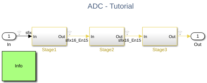
Final System-Level Model
This example shows you how to put together all the previous steps of the ADC tutorial in a single model to better allow system-simulation and performance estimation.
The MSADCTutorial_Model3_1 model allows the simulation of the ADC using the different implementations created in the System-Level Model of DSM ADC example.
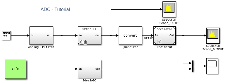
model = 'MSADCTutorial_Model3_1.slx';
open_system(model);
sim(model);
For the analog filter, you use can a subsystem to gather the Bode Plot and the filter model in the same diagram. This makes easier to understand which subsystem is linearized and reduce the cluttering at the top-level. The two available models of the filter are stored in a custom library using a variant subsystem. The user can toggle which filter model to use by right-clicking on the filter block in the model testbench and selecting a different active variant.
You can inspect the analog filter library:
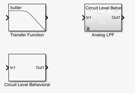
filterLibrary = 'AnalogFilter.slx';
open_system(filterLibrary);
For the data converter you can use a similar approach. The three available models of the data converter are stored in a custom library using a variant subsystem. The user can toggle which converter model to use by right clicking on the ADC block in the testbench and selecting a different active variant.
You can inspect the data converter library:

converterLibrary = 'DeltaSigma.slx';
open_system(converterLibrary);
For the decimator filter you can use model referencing in order to choose a different solver (fixed-step discrete) for the digital filter and for the generation of HDL code. With reference models you can divide Simulink models over multiple files, and it is therefore recommended when collaborating with multiple team members on the same project.
DecimatorModel = 'Decimator.slx';
open_system(DecimatorModel);
ADC AC Measurements
You can use the Mixed-Signal Blockset™ ADC Tesbench block to characterize the ADC AC performance.
In the MSADCTutorial_Model3_2 model, you find the testbench block configured for AC measurements highlighted in purple. This helps you in veryfing the nonlinearity and the noise performance of the ADC. With the ADC Testbench you can compute the SNR and the ENOB. You can verify that the testbench provides the expected theoretical results by comparing with the SNR and ENOB as function of modulator order and OSR as described in [1] and reported in the table below:
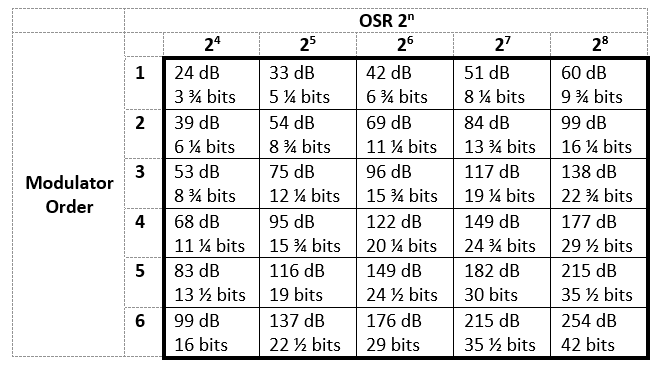
Since the ADC model is behavioral and the adc ready signal is not properly generated, the measured conversion delay is incorrect.

model = 'MSADCTutorial_Model3_2.slx';
open_system(model);
sim(model);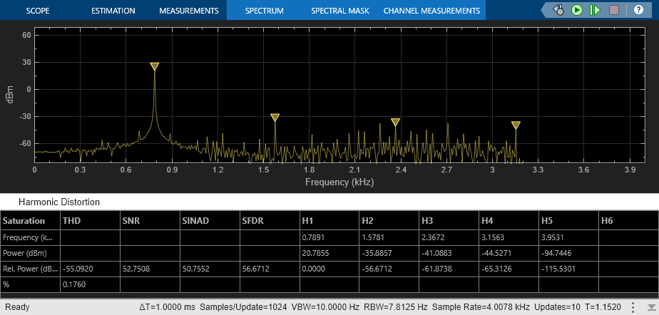
You can now toggle the modulator order, and revalidate that results for a second order modulator.

set_param('MSADCTutorial_Model3_2/ADC','LabelModeActiveChoice','Variant2');
sim(model);

Conclusion
You have seen how to build a system-level model connecting together all the design elements developed at the previous steps of this tutorial. You have seen how to use library and configurable subsystems to enable the ability to toggle between different views (abstraction level) of the same block. You have used a reference model to split a Simulink model over multiple files using a different configuration.
References
[1] Dave Van Ess. "Signals From Noise: Calculating Delta-Sigma SNRs."