System-Level Model of DSM ADC
This example shows how to develop a system-level model of a 2nd-order DSM (delta-sigma modulator) ADC. This example consists of three steps:
Analog Anti-Aliasing Filter Design
You can use a 1st-order DSM as a starting point to design an anti-aliasing filter. Open the model MSADCTutorial_Model1_1 attached with this example. The model uses Simscape™ to describe the analog filter in the domain of voltages and currents using RLC components and operational amplifiers.

model = 'MSADCTutorial_Model1_1.slx';
open_system(model);
sim(model);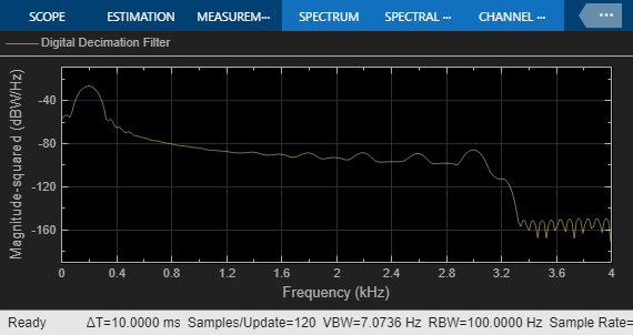

Circuit-Level Behavioral Model of Analog Filter
Model the analog filter using lumped RLC components and operational amplifiers.
Double-click and open the Circuit-Level Analog Filter subsystem. The subsystem uses a 3rd-order Butterworth filter which is implemented using a tree-stage structure. The filter is active with a positive gain.

open_system([gcs '/Circuit-Level Analog Filter']);If you have specific design information about the circuit level implementation of your filter, you can decide to include imperfections of the op-amp implementation such as impedance mismatch, finite slew rate, noise, finite gain. Simscape Electrical™ provides more accurate models, and even transistor level models, to model analog systems at the lower level of abstraction.
Validation of Circuit-Level Implementation
Although time domain simulation of the filter output looks correct, this does not gives us confidence that the filter actually implements the correct transfer function.
You can use a discrete transfer function estimator block from DSP System Toolbox™, however this would require sampling the input and output signals with a fixed sample time, which could be error prone.
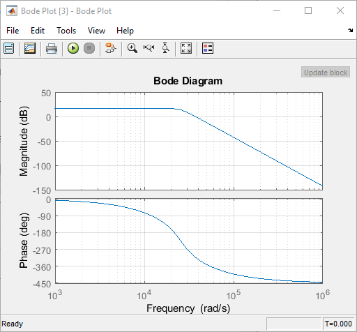
A simpler alternative for the validation of the transfer function consists in using the Bode Plot from Simulink Control Design, as used in the model MSADCTutorial_Model1_2 attached with this example.
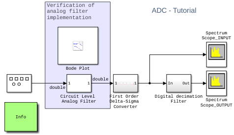
model = 'MSADCTutorial_Model1_2.slx';
open_system(model);
sim(model);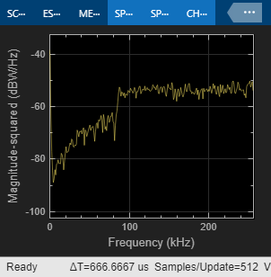

The Bode Plot block computes the magnitude and phase transfer function of the analog filter by linearizing the block at a specific simulation time. The input signal of the filter provides the input perturbation. The output signal of the filter provides the measured output. The Bode Plot block computes the transfer function of the subsystem in between the input perturbation and the output measurement.
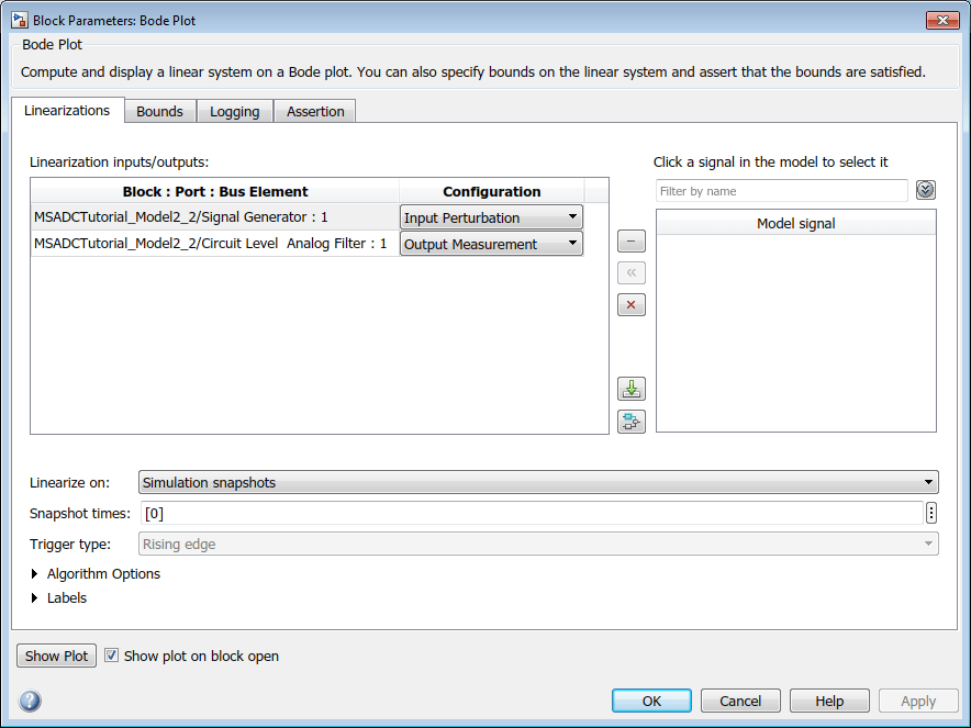
In this case, you have linearized the block at time 0. As this particular subsystem is time-invariant, you can choose any arbitrary time to linearize it. As the Bode Plot block has an impact on the simulation speed, after you have validated the circuit level implementation you might want to remove it, or comment it out.
Converter Design
This section of the example refines the model of the delta-sigma converter and provide a more realistic description and a possible switched-capacitor implementation.
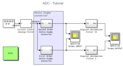
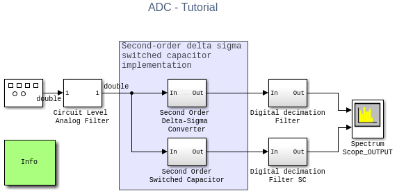
Implement the converter using a 2nd-order delta-sigma modulator. This design allows you to achieve a better in-band noise performance. Start by developing a high-level behavioral model such as MSADCTutorial_Model1_3 and comparing the results to the 1st-order model.
model = 'MSADCTutorial_Model1_3.slx';
open_system(model);
sim(model);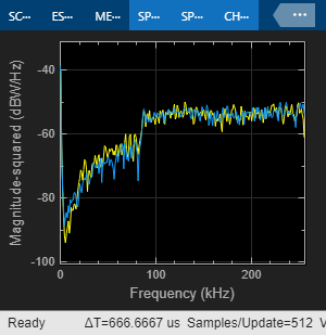
Open the Second Order Delta-Sigma Converter to inspect the behaviorial model.
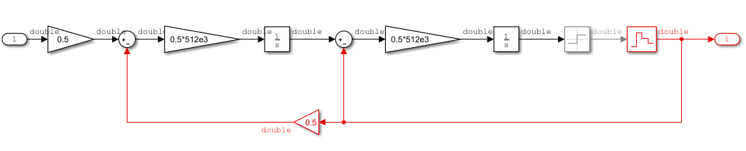
open_system([gcs '/Second Order Delta-Sigma Converter']);Second-Order Delta-Sigma Converter Circuit-Level Model
Use a possible implementation of the delta-sigma converter using switched capacitors. In the model MSADCTutorial_Model1_4 attached with this example, Simscape Electrical is used to provide a differential implementation of the delta sigma where the clocks are explicitly modelled. Also the imperfections of the op-amps are modelled such as the bandwidth, impedance, slew rate, and saturation.
model = 'MSADCTutorial_Model1_4.slx';
open_system(model);
sim(model);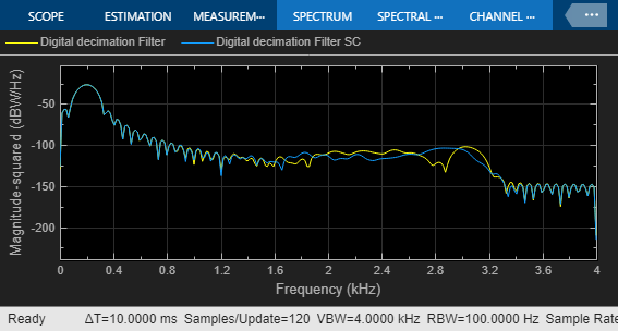
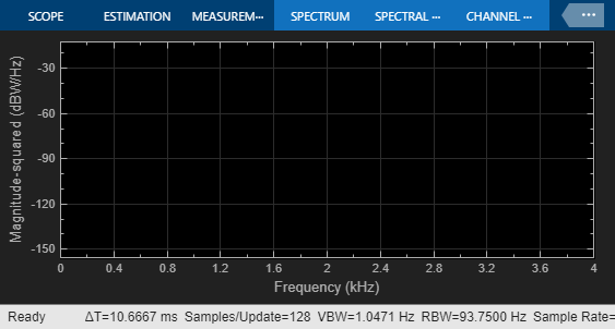
The simulation speed is now slower, due to the higher complexity of the Second Order Switched Capacitor subsystem. The output spectrum shows a good fit when compared with the reference second order behavioral model, however the imperfections in the converter implementation degrade the noise performance compared to the ideal reference model.
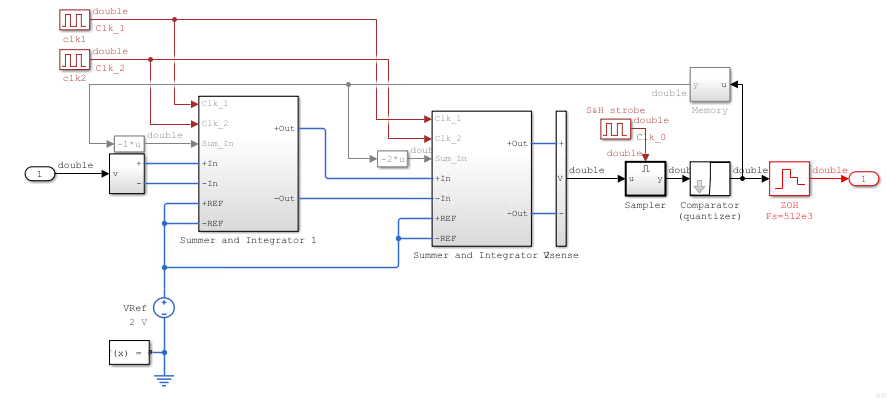
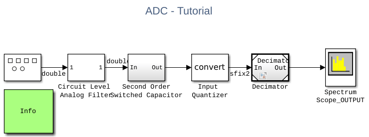
open_system([gcs '/Second Order Switched Capacitor']);Digital Decimation Filter Design
This section of the example converts the digital decimation filter from floating point to fixed-point. The model of the digital filter that uses integer arithmetic allows you to automatically generate synthesizable HDL code. Last, you generate synthesizable HDL, and validate the results using cosimulation with Cadence® Incisive.
The multi-rate multi-stage digital filter has been designed with filterBuilder function.
The filter specifications are the following:
Response type:
LowpassImpulse response:
FIRFilter type:
DecimatorDecimation factor:
64Input data rate:
64*8kHzPassband frequency:
3kHzStopband frequency:
3.3kHzPassband ripple:
1dBStopband attenuation:
80dBDesign method:
Multistage equiripple
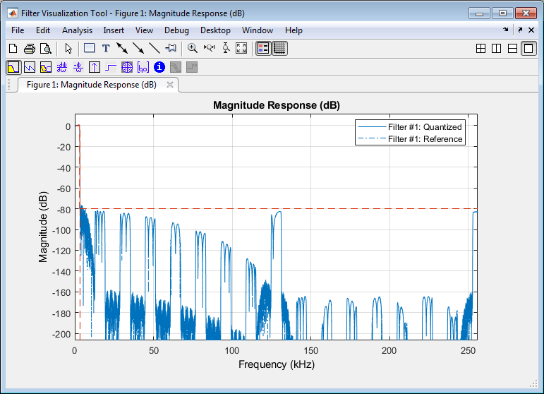
You can inspect the filter properties and its response here:
load MSADCTutorial_DigitalFilter.mat;
filterBuilder(Hlp);
Digital Filter Fixed-Point Conversion
If you inspect the tab Data Types in the filter builder project, you see that the filter has been initially designed using double floating point accuracy by setting Arithmetic to Double precision. To convert the filter to using integer arithmetic, set Arithmetic to Fixed point.
When converting the filter to fixed-point you have control on the data types of input/output signals, the filter coefficients, and also the internal variables (signals) of the filter.
Start with an initial conversion using mostly default parameters as you can see in this figure:
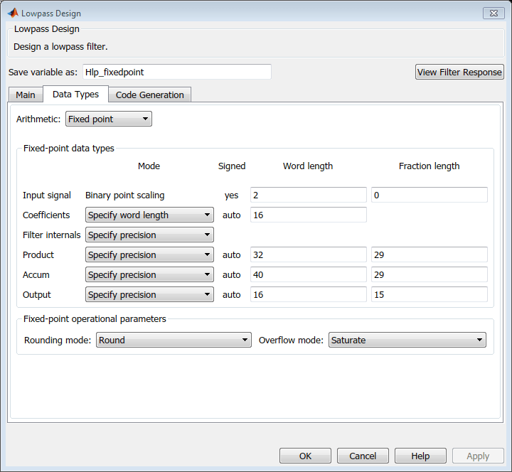
Although the converted filter transfer function is not fully compliant to the given specifications, you can consider it sufficiently accurate to achieve the desired performance.
The current filter implementation is now stored in the MATLAB variable Hlp_fixedpoint. You can generate a Simulink model for the filter and add this block in the system-level model you have been using.
filterBuilder(Hlp_fixedpoint);
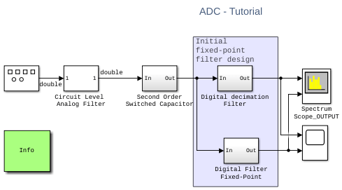
Verification of Digital Filter Fixed-Point Implementation
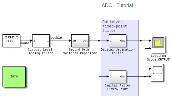
You can now simulate the new implementation of the digital filter and verify its performance using the model MSADCTutorial_Model1_5.
model = 'MSADCTutorial_Model1_5.slx';
open_system(model);
sim(model);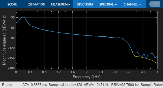
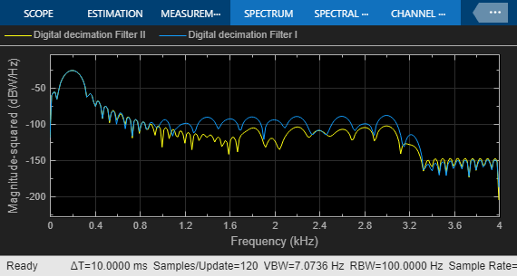
After running the model for just a few cycles of the input sinusoidal signal, you can verify that the results of fixed-point and floating point filter models show good agreement both in the time- and frequency-domains, although the quantization effect is visible in the stopband of the filter.
Although the simulation results give you confidence that the fixed-point model is correct overall, this does not provide you with an insightful analysis and it does not help you in identifying opportunities for optimizing the fractional length.
open_system([gcs '/Digital Filter Fixed-Point']);Fixed-Point Optimization
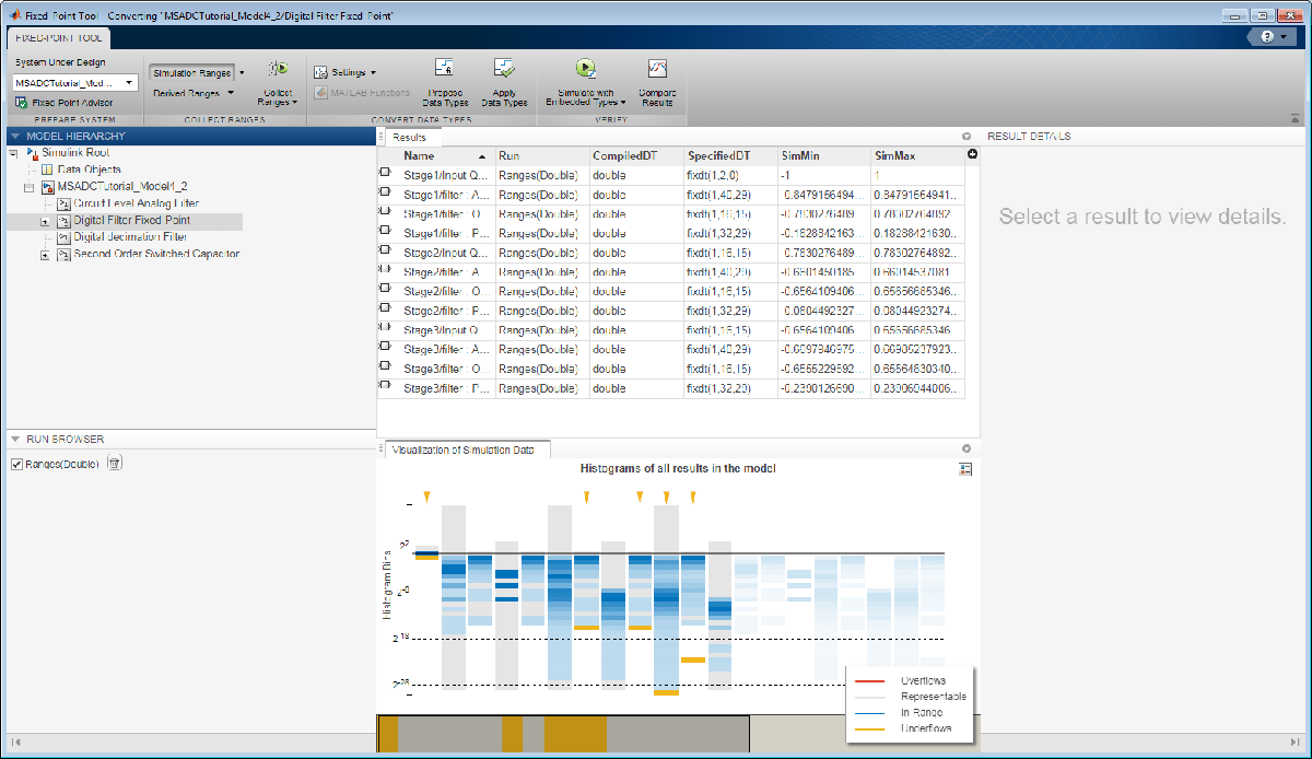
You can check if the fixed-point fraction length is optimal by launching the Fixed-Point Tool. Right click on the existing fixed-point implementation of the filter and launch Fixed-Point Tool.
Select the fixed-point digital filter implementation in the System Under Design pane, change its settings to log minimal maximum and overflows, and collect the signal dynamic ranges via simulation. The fixed-point signals are automatically converted to double floating point to gather data and determine the true dynamic range of the signals.
When the simulation is finished, the logged data is visualized using histograms, providing a good idea of the quality of the results.
After logging the dynamic range of the simulation data, you can use this data to propose new data types optimized for these operating conditions. You can inspect, eventually modify, and apply the proposed data types. The resulting model is similar to the model MSADCTutorial_Model1_6.
model = 'MSADCTutorial_Model1_6.slx';
open_system(model);
sim(model);
HDL Code Generation for Digital Filter
The fixed-point model of the digital filter provides a bit-accurate representation of the filter. You can now proceed to automatically generate synthesizable HDL code for the filter.
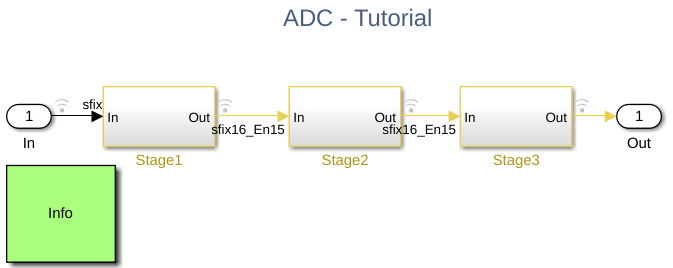
One prerequisite for HDL code generation is that the Simulink model must use a fixed-step discrete time solver. As the ADC model uses continuous time signals, you cannot simply change the solver configuration. You can use model referencing to solve this issue, and save the digital filter in a separate Decimator model.
model = 'Decimator.slx';
open_system(model);
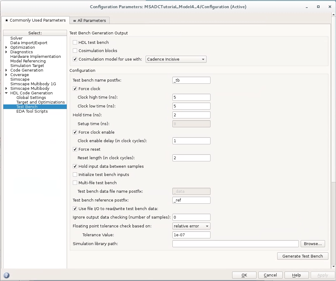
myConfigObj = getActiveConfigSet(gcs);
openDialog(myConfigObj)As you can see, this model uses a fixed-step discrete solver with a configuration that is compatible with HDL (Verilog) code generation.
The top-level model MSADCTutorial_Model1_7 referencing the decimator implementation can be seen here:
testbench = 'MSADCTutorial_Model1_7.slx';
open_system(testbench);
sim(testbench);
### Searching for referenced models in model 'MSADCTutorial_Model1_7'. ### Total of 1 models to build. ### Starting serial model build. ### Successfully updated the model reference simulation target for: Decimator Build Summary Model reference simulation targets: Model Build Reason Status Build Duration ===================================================================================================== Decimator Target (Decimator_msf.mexw64) did not exist. Code generated and compiled. 0h 0m 50.36s 1 of 1 models built (0 models already up to date) Build duration: 0h 0m 52.617s

You can use the Logic Analyzer app to inspect the results at each stage of decimation filter. For more information, see Inspect and Measure Transitions Using the Logic Analyzer
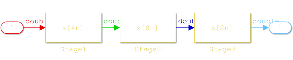
Right click on the reference model of the digital filter to generate HDL code. A report is automatically created including bidirectional traceability links between the modeling features and the automatically generated code. You can further optimize the generated code by specifying HDL properties of each filter stage. For example, you can specify a fully parallel, or a fully serial implementation, add distributed pipelines, or share resources.
makehdl([gcs '/Decimator'], 'TargetDirectory','./work/hdlsrc');
### Working on the model MSADCTutorial_Model1_7
### Generating HDL for MSADCTutorial_Model1_7/Decimator
### Using the config set for referenced model Decimator for HDL code generation parameters.
### Begin compilation of the model 'MSADCTutorial_Model1_7'...
### Searching for referenced models in model 'MSADCTutorial_Model1_7'.
### Total of 1 models to build.
### Starting serial model build.
### Model reference simulation target for Decimator is up to date.

Build Summary

0 of 1 models built (1 models already up to date)
Build duration: 0h 0m 2.9698s
### Begin compilation of the model 'Decimator'...
### Running HDL checks on the model 'Decimator'.
### Begin compilation of the model 'Decimator'...
### Working on the model 'Decimator'...
### Working on... GenerateModel
### Begin model generation 'gm_Decimator'...
### Rendering DUT with optimization related changes (IO, Area, Pipelining)...
### Model generation complete.
### Generated model saved at .\work\hdlsrc\MSADCTutorial_Model1_7\gm_Decimator.slx
### Begin Verilog Code Generation for 'Decimator'.
### Begin Verilog Code Generation for 'Decimator_tc'.
### Working on Decimator_tc as .\work\hdlsrc\MSADCTutorial_Model1_7\Decimator_tc.v.
### Code Generation for 'Decimator_tc' completed.
### Working on Decimator/Stage1/filter as .\work\hdlsrc\MSADCTutorial_Model1_7\filter.v.
### Working on Decimator/Stage1 as .\work\hdlsrc\MSADCTutorial_Model1_7\Stage1.v.
### Working on Decimator/Stage2/filter as .\work\hdlsrc\MSADCTutorial_Model1_7\filter_block.v.
### Working on Decimator/Stage2 as .\work\hdlsrc\MSADCTutorial_Model1_7\Stage2.v.
### Working on Decimator/Stage3/filter as .\work\hdlsrc\MSADCTutorial_Model1_7\filter_block1.v.
### Working on Decimator/Stage3 as .\work\hdlsrc\MSADCTutorial_Model1_7\Stage3.v.
### Working on Decimator as .\work\hdlsrc\MSADCTutorial_Model1_7\Decimator.v.
### Code Generation for 'Decimator' completed.
### Generating HTML files for code generation report at index.html
### Creating HDL Code Generation Check Report Decimator_report.html
### HDL check for 'Decimator' complete with 0 errors, 1 warnings, and 0 messages.
### Creating HDL Code Generation Check Report MSADCTutorial_Model1_7_report.html
### HDL check for 'MSADCTutorial_Model1_7' complete with 0 errors, 0 warnings, and 1 messages.
### HDL code generation complete.
Generate Cosimulation Model
After HDL code generation, you can validate the results in Cadence Incisive leveraging cosimulation.
To complete the cosimulation step, you run the model using the Linux® operating system, and you need a running installation of Cadence Incisive or Cadence Xcelium.
Cadence Incisive™
Cadence Xcelium™
You can configure which third party tool to leverage for cosimulation from the HDL configuration window pane "testbenches".
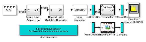
The final testbench looks like the following image, where the top branch represents our reference model, and the bottom branch is actually simulated in Incisive. Results plotted on the right show that there is no difference between the results of the reference model and of the cosimulation one.
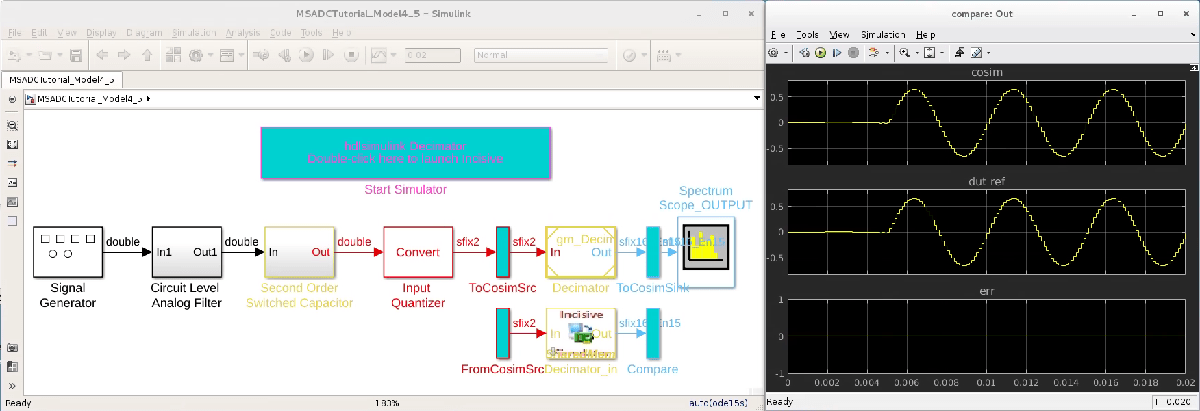
You can also inspect results in Incisive:
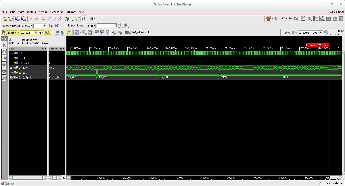
If you are running this tutorial on a Linux machine with a valid Incisive installation, you can just open and run the cosimulation model MSADCTutorial_Model1_8.
testbench = 'MSADCTutorial_Model1_8.slx';
open_system(testbench);
Summary: Converter Design
You have created a realistic model of a 2nd-order DSM ADC starting from a simple 1st-order DSM ADC model. You have generated synthesizable HDL code and validated the results using cosimulation with Cadence Incisive.