Main Content

istft

Inverse short-time Fourier transform

Description

x = istft(s) returns the Inverse Short-Time Fourier Transform (ISTFT) of s.

example

x = istft(s,fs) returns the ISTFT of s using sample rate fs.

x = istft(s,ts) returns the ISTFT using sample time ts.

example

x = istft(___,Name,Value) specifies additional options using name-value pair arguments. Options include the FFT window length and number of overlapped samples. These arguments can be added to any of the previous input syntaxes.

example

[x,t] = istft(___) returns the signal times at which the ISTFT is evaluated.

Examples

collapse all

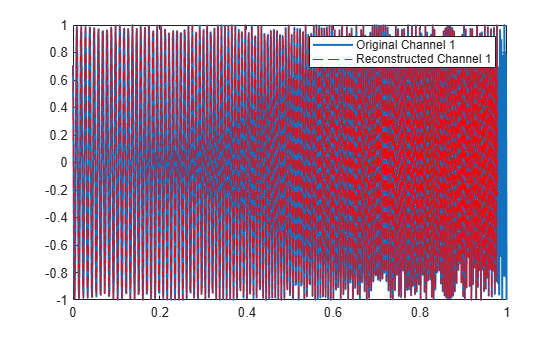
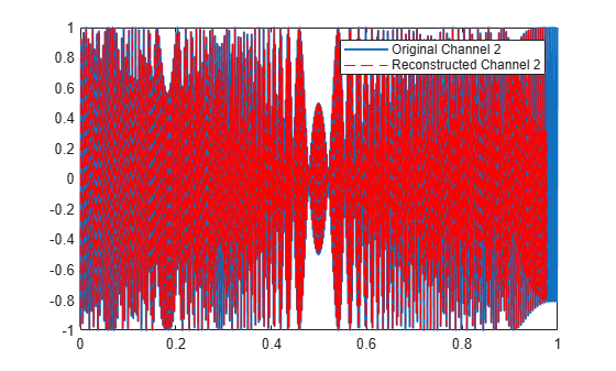
Generate a three-channel signal consisting of three different chirps sampled at 1 kHz for 1 second.

  1. The first channel consists of a concave quadratic chirp with instantaneous frequency 100 Hz at t = 0 and crosses 300 Hz at t = 1 second. It has an initial phase equal to 45 degrees.

  2. The second channel consists of a convex quadratic chirp with instantaneous frequency 200 Hz at t = 0 and crosses 600 Hz at t = 1 second.

  3. The third channel consists of a logarithmic chirp with instantaneous frequency 300 Hz at t = 0 and crosses 500 Hz at t = 1 second.

Compute the STFT of the multichannel signal using a periodic Hamming window of length 256 and an overlap length of 15 samples.

fs = 1e3;
t = 0:1/fs:1-1/fs;
x = [chirp(t,100,1,300,'quadratic',45,'concave');
      chirp(t,200,1,600,'quadratic',[],'convex');
      chirp(t,300,1,500,'logarithmic')]'; 
  
[S,F,T] = stft(x,fs,'Window',hamming(256,'periodic'),'OverlapLength',15);

Plot the original and reconstructed versions of the first and second channels.

[ix,ti] = istft(S,fs,'Window',hamming(256,'periodic'),'OverlapLength',15);

plot(t,x(:,1)','LineWidth',1.5)
hold on
plot(ti,ix(:,1)','r--')
hold off
legend('Original Channel 1','Reconstructed Channel 1')

plot(t,x(:,2)','LineWidth',1.5)
hold on
plot(ti,ix(:,2)','r--')

legend('Original Channel 2','Reconstructed Channel 2')

The phase vocoder performs time stretching and pitch scaling by transforming the audio in the frequency domain. This diagram shows the operations involved in the phase vocoder implementation.

The phase vocoder takes the STFT of a signal with an analysis window of hop size R1 and then performs an ISTFT with a synthesis window of hop size R2. The vocoder thus takes advantage of the WOLA method. To time stretch a signal, the analysis window uses a larger number of overlap samples than the synthesis. As a result, there are more samples at the output than at the input (NS,Out>NS,In), although the frequency content remains the same. Now, you can pitch scale this signal by playing it back at a higher sample rate, which produces a signal with the original duration but a higher pitch.

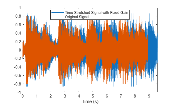
Load an audio file containing a fragment of Handel's "Hallelujah Chorus" sampled at 8192 Hz.

load handel

Design a root-Hann window of length 512. Set analysis overlap length as 192 and synthesis overlap length as 166.

wlen = 512;
win = sqrt(hann(wlen,'periodic'));
noverlapA = 192;
noverlapS = 166;

Implement the phase vocoder by using an analysis window of overlap 192 and a synthesis window of overlap 166.

S = stft(y,Fs,'Window',win,'OverlapLength',noverlapA);
iy = istft(S,Fs,'Window',win,'OverlapLength',noverlapS);

%To hear, type soundsc(y,Fs), pause(10), soundsc(iy,Fs);

If the analysis and synthesis windows are the same but the overlap length is changed, there will be an additional gain/loss that you will need to adjust. This is a common approach to implementing a phase vocoder.

Calculate the hop ratio and use it to adjust the gain of the reconstructed signal. Also calculate frequency of pitch-shifted data using the hop ratio.

hopRatio = (wlen-noverlapS)/(wlen-noverlapA);
iyg = iy*hopRatio;
Fp = Fs*hopRatio;

%To hear, type soundsc(iyg,Fs), pause(15), soundsc(iyg,Fp);

Plot the original signal and the time stretched signal with fixed gain.

plot((0:length(iyg)-1)/Fs,iyg,(0:length(y)-1)/Fs,y)
xlabel('Time (s)')
xlim([0 (length(iyg)-1)/Fs])
legend('Time Stretched Signal with Fixed Gain','Original Signal','Location','best')

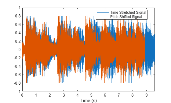
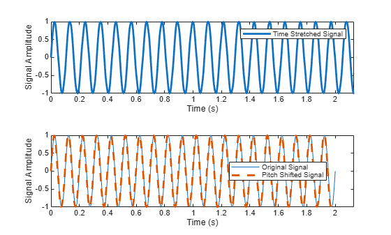
Compare the time-stretched signal and the pitch shifted signal on the same plot.

plot((0:length(iy)-1)/Fs,iy,(0:length(iy)-1)/Fp,iy)
xlabel('Time (s)')
xlim([0 (length(iyg)-1)/Fs])
legend('Time Stretched Signal','Pitch Shifted Signal','Location','best') 

To better understand the effect of pitch shifting data, consider the following sinusoid of frequency Fs over 2 seconds.

t = 0:1/Fs:2;
x = sin(2*pi*10*t);

Calculate the short-time Fourier transform and the inverse short-time Fourier transform with overlap lengths 192 and 166 respectively.

Sx = stft(x,Fs,'Window',win,'OverlapLength',noverlapA);
ix = istft(Sx,Fs,'Window',win,'OverlapLength',noverlapS);

Plot the original signal on one plot and the time-stretched and pitch shifted signal on another.

tiledlayout(2,1)
nexttile
plot((0:length(ix)-1)/Fs,ix,'LineWidth',2) 
xlabel('Time (s)')
ylabel('Signal Amplitude')
xlim([0 (length(ix)-1)/Fs])
legend('Time Stretched Signal') 
nexttile
plot((0:length(x)-1)/Fs,x)
hold on
plot((0:length(ix)-1)/Fp,ix,'--','LineWidth',2)
legend('Original Signal','Pitch Shifted Signal','Location','best')
hold off
xlabel('Time (s)')
ylabel('Signal Amplitude')
xlim([0 (length(ix)-1)/Fs])

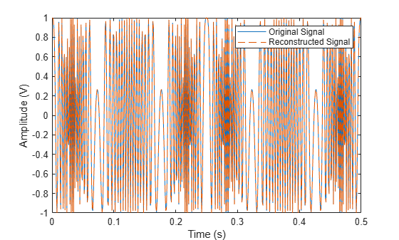
Generate a complex sinusoid of frequency 1 kHz and duration 2 seconds.

fs = 1e3;
ts = 0:1/fs:2-1/fs;

x = exp(2j*pi*100*cos(2*pi*2*ts));

Design a periodic Hann window of length 100 and set the number of overlap samples to 75. Check the window and overlap length for COLA compliance.

nwin = 100;
win = hann(nwin,'periodic');
noverlap = 75;

tf = iscola(win,noverlap)
tf = logical
   1

Zero-pad the signal to remove edge-effects. To avoid truncation, pad the input signal with zeros such that

length(xZero)-noverlapnwin-noverlapSignal length minus overlap over window length minus overlap

is an integer. Set the FFT length to 128. Compute the short-time Fourier transform of the complex signal.

nPad = 100;
xZero = [zeros(1,nPad) x zeros(1,nPad)];
fftlen = 128;
s = stft(xZero,fs,'Window',win,'OverlapLength',noverlap,'FFTLength',fftlen);

Calculate the inverse short-time Fourier transform and remove the zeros for perfect reconstruction.

[is,ti] = istft(s,fs,'Window',win,'OverlapLength',noverlap,'FFTLength',fftlen);
is(1:nPad) = [];
is(end-nPad+1:end) = [];
ti = ti(1:end-2*nPad);

Plot the real parts of the original and reconstructed signals. The imaginary part of the signal is also reconstructed perfectly.

plot(ts,real(x))
hold on
plot(ti,real(is),'--')
xlim([0 0.5])
xlabel('Time (s)')
ylabel('Amplitude (V)')
legend('Original Signal','Reconstructed Signal') 
hold off

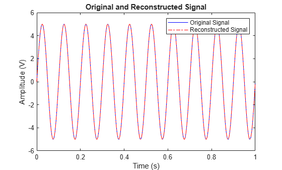
Generate a sinusoid sampled at 2 kHz for 1 second.

fs = 2e3;
t = 0:1/fs:1-1/fs;
x = 5*sin(2*pi*10*t);

Design a periodic Hamming window of length 120. Check the COLA constraint for the window with an overlap of 80 samples. The window-overlap combination is COLA compliant.

win = hamming(120,'periodic');
noverlap = 80;
tf = iscola(win,noverlap)
tf = logical
   1

Set the FFT length to 512. Compute the short-time Fourier transform.

fftlen = 512;
s = stft(x,fs,'Window',win,'OverlapLength',noverlap,'FFTLength',fftlen);

Calculate the inverse short-time Fourier transform.

[X,T] = istft(s,fs,'Window',win,'OverlapLength',noverlap,'FFTLength',fftlen,'Method','ola','ConjugateSymmetric',true);

Plot the original and reconstructed signals.

plot(t,x,'b')
hold on
plot(T,X,'-.r')
xlabel('Time (s)')
ylabel('Amplitude (V)')
title('Original and Reconstructed Signal')
legend('Original Signal','Reconstructed Signal')
hold off

Input Arguments

collapse all

Short-time Fourier transform, specified as a matrix or a 3-D array. For single-channel signals, specify s as a matrix with time increasing across the columns and frequency increasing down the rows. For multichannel signals, specify s as a 3-D array with the third dimension corresponding to the channels. The frequency and time vectors are obtained as outputs of stft.

Note

If you want x and s to be the same length, the value of (length(x)-noverlap)/(length(window)-noverlap) must be an integer. Use Window to specify the length of window and OverlapLength to specify noverlap.

Data Types: double | single
Complex Number Support: Yes

Sample rate in hertz, specified as a positive scalar.

Data Types: double | single

Sample time, specified as a duration scalar.

Example: seconds(1) is a duration scalar representing a 1-second time difference between consecutive signal samples.

Data Types: duration

Name-Value Arguments

Specify optional pairs of arguments as Name1=Value1,...,NameN=ValueN, where Name is the argument name and Value is the corresponding value. Name-value arguments must appear after other arguments, but the order of the pairs does not matter.

Example: istft(s,Window=win,OverlapLength=50,FFTLength=128) windows the data using the window win, with 50 samples overlap between adjoining segments and 128 DFT points.

Before R2021a, use commas to separate each name and value, and enclose Name in quotes.

Example: istft(s,'Window',win,'OverlapLength',50,'FFTLength',128) windows the data using the window win, with 50 samples overlap between adjoining segments and 128 DFT points.

Windowing function, specified as a vector. If you do not specify the window or specify it as empty, the function uses a periodic Hann window of length 128. The length of Window must be greater than or equal to 2.

For a list of available windows, see Windows.

Example: hann(N+1) and (1-cos(2*pi*(0:N)'/N))/2 both specify a Hann window of length N + 1.

Data Types: double | single

Number of overlapped samples, specified as a nonnegative integer smaller than the length of window. If you omit OverlapLength or specify it as empty, it is set to the largest integer less than 75% of the window length, which turns out to be 96 samples for the default Hann window.

Data Types: double | single

Number of DFT points, specified as a positive integer greater than or equal to the length of the window. To achieve perfect time-domain reconstruction, you must set the number of DFT points to match that used in stft.

Data Types: double | single

Method of overlap-add, specified as one of these:

  • "wola" — Weighted overlap-add

  • "ola" — Overlap-add

Conjugate symmetry of the original signal, specified as true or false. If this option is set to true, istft assumes that the input s is symmetric, otherwise no symmetric assumption is made. When s is not exactly conjugate symmetric due to round-off error, setting the name-value pair to true ensures that the STFT is treated as if it were conjugate symmetric. If s is conjugate symmetric, then the inverse transform computation is faster, and the output is real.

STFT frequency range, specified as "centered", "twosided", or "onesided".

  • "centered" — Treat s as a two-sided, centered STFT. If nfft is even, then s is considered to be computed over the interval (–π, π] rad/sample. If nfft is odd, then s is considered to be computed over the interval (–π, π) rad/sample. If you specify time information, then the intervals are (–fs, fs/2] cycles/unit time and (–fs, fs/2) cycles/unit time, respectively, where fs is the sample rate.

  • "twosided" — Treat s as a two-sided STFT computed over the interval [0, 2π) rad/sample. If you specify time information, then the interval is [0, fs) cycles/unit time.

  • "onesided" — Treat s as a one-sided STFT. If nfft is even, then s is considered to be computed over the interval [0, π] rad/sample. If nfft is odd, then s is considered to be computed over the interval [0, π) rad/sample. If you specify time information, then the intervals are [0, fs/2] cycles/unit time and [0, fs/2) cycles/unit time, respectively, where fs is the sample rate.

    Note

    When this argument is set to "onesided", istft assumes the values in the positive Nyquist range were computed without conserving the total power.

For an example, see STFT Frequency Ranges.

Data Types: char | string

Input time dimension, specified as "acrosscolumns" or "downrows". If this value is set to "downrows", istft assumes that the time dimension of s is down the rows and the frequency is across the columns. If this value is set to "acrosscolumns", the function istft assumes that the time dimension of s is across the columns and frequency dimension is down the rows.

Output Arguments

collapse all

Reconstructed signal in the time domain, returned as a vector or a matrix.

Data Types: single | double

Time instants, returned as a vector.

  • If a sample rate fs is provided, then t contains time values in seconds.

  • If a duration ts is provided, then t has the same time format as the input duration and is a duration array.

  • If no time information is provided, then t contains sample numbers.

Data Types: double | single

More About

collapse all

Inverse Short-Time Fourier Transform

The inverse short-time Fourier transform is computed by taking the IFFT of each DFT vector of the STFT and overlap-adding the inverted signals. The ISTFT is calculated as follows.

x(n)=1/21/2m=Xm(f)ej2πfndf=m=1/21/2Xm(f)ej2πfndf=m=xm(n),

where R is the hop size between successive DFTs, Xm is the DFT of the windowed data centered about time mR, and xm(n)=x(n)g(nmR). The inverse STFT is a perfect reconstruction of the original signal as long as m=ga+1(nmR)=cn, where the analysis window g(n) was used to window the original signal and c is a constant. This figure depicts the steps in reconstructing the original signal.

Constant Overlap-Add (COLA) Constraint

To ensure successful reconstruction of nonmodified spectra, the analysis window must satisfy the COLA constraint. In general, if the analysis window satisfies the condition m=ga+1(nmR)=cn,, the window is considered to be COLA-compliant. Additionally, COLA compliance can be described as either weak or strong.

  • Weak COLA compliance implies that the Fourier transform of the analysis window has zeros at frame-rate harmonics such that

    G(fk)=0,k=1,2,,R1,fkkR.

    Alias cancellation is disturbed by spectral modifications. Weak COLA relies on alias cancellation in the frequency domain. Therefore, perfect reconstruction is possible using weakly COLA-compliant windows as long as the signal has not undergone any spectral modifications.

  • For strong COLA compliance, the Fourier transform of the window must be bandlimited consistently with downsampling by the frame rate such that

    G(f)=0,f12R.

    This equation shows that no aliasing is allowed by the strong COLA constraint. Additionally, for strong COLA compliance, the value of the constant c must equal 1. In general, if the short-time spectrum is modified in any way, a stronger COLA compliant window is preferred.

You can use the iscola function to check for weak COLA compliance. The number of summations used to check COLA compliance is dictated by the window length and hop size. In general, it is common to use a=1 in m=ga+1(nmR)=cn, for weighted overlap-add (WOLA), and a=0 for overlap-add (OLA). By default, istft uses the WOLA method, by applying a synthesis window before performing the overlap-add method.

In general, the synthesis window is the same as the analysis window. You can construct useful WOLA windows by taking the square root of a strong OLA window. You can use this method for all nonnegative OLA windows. For example, the root-Hann window is a good example of a WOLA window.

Perfect Reconstruction

In general, computing the STFT of an input signal and inverting it does not result in perfect reconstruction. If you want the output of ISTFT to match the original input signal as closely as possible, the signal and the window must satisfy the following conditions:

  • Input size — If you invert the output of stft using istft and want the result to be the same length as the input signal x, the value of

    k = NxLML

    must be an integer. In the equation, Nx is the length of the signal, M is the length of the window, and L is the overlap length.

  • COLA compliance — Use COLA-compliant windows, assuming that you have not modified the short-time Fourier transform of the signal.

  • Padding — If the length of the input signal is such that the value of k is not an integer, zero-pad the signal before computing the short-time Fourier transform. Remove the extra zeros after inverting the signal.

References

[1] Crochiere, R. E. "A Weighted Overlap-Add Method of Short-Time Fourier Analysis/Synthesis." IEEE Transactions on Acoustics, Speech and Signal Processing. Vol. 28, Number 1, Feb. 1980, pp. 99–102.

[2] Gotzen, A. D., N. Bernardini, and D. Arfib. "Traditional Implementations of a Phase-Vocoder: The Tricks of the Trade." Proceedings of the COST G-6 Conference on Digital Audio Effects (DAFX-00), Verona, Italy, Dec 7–9, 2000.

[3] Griffin, Daniel W., and Jae S. Lim. "Signal Estimation from Modified Short-Time Fourier Transform." IEEE Transactions on Acoustics, Speech and Signal Processing. Vol. 32, Number 2, April 1984, pp. 236–243.

[4] Portnoff, M. R. "Time-Frequency Representation of Digital Signals and Systems Based on Short-Time Fourier analysis." IEEE Transactions on Acoustics, Speech and Signal Processing. Vol. 28, Number 1, Feb 1980, pp. 55–69.

[5] Smith, Julius Orion. Spectral Audio Signal Processing. https://ccrma.stanford.edu/~jos/sasp/, online book, 2011 edition, accessed Nov. 2018.

[6] Sharpe, Bruce. Invertibility of Overlap-Add Processing. https://gauss256.github.io/blog/cola.html, accessed July 2019.

Extended Capabilities

Version History

Introduced in R2019a