pspectrum
Analyze signals in the frequency and time-frequency domains
Syntax
Description
p = pspectrum(x)x.
If
xis a vector or a timetable with a vector of data, then it is treated as a single channel.If
xis a matrix, a timetable with a matrix variable, or a timetable with multiple vector variables, then the spectrum is computed independently for each channel and stored in a separate column ofp.
p = pspectrum(___,Name=Value)
Examples
Generate 128 samples of a two-channel complex sinusoid.
The first channel has unit amplitude and a normalized sinusoid frequency of rad/sample
The second channel has an amplitude of and a normalized frequency of rad/sample.
Compute and plot the power spectrum of each channel. Zoom in on the frequency range from rad/sample to rad/sample. pspectrum scales the spectrum so that, if the frequency content of a signal falls exactly within a bin, its amplitude in that bin is the true average power of the signal. For a complex exponential, the average power is the square of the amplitude. Verify by computing the discrete Fourier transform of the signal. For more details, see Measure Power of Deterministic Periodic Signals.
N = 128;
x = [1 1/sqrt(2)].*exp(1j*pi./[4;2]*(0:N-1)).';

[p,f] = pspectrum(x);

plot(f/pi,p)
hold on
stem(0:2/N:2-1/N,abs(fft(x)/N).^2)
hold off
axis([0.15 0.6 0 1.1])
legend("Channel "+[1;2]+", "+["pspectrum" "fft"])
grid

Generate a sinusoidal signal sampled at 1 kHz for 296 milliseconds and embedded in white Gaussian noise. Specify a sinusoid frequency of 200 Hz and a noise variance of 0.1². Store the signal and its time information in a MATLAB® timetable.
Fs = 1000;
t = (0:1/Fs:0.296)';
x = cos(2*pi*t*200)+0.1*randn(size(t));
xTable = timetable(seconds(t),x);
Compute the power spectrum of the signal. Express the spectrum in decibels and plot it.
[pxx,f] = pspectrum(xTable);

plot(f,pow2db(pxx))
grid on
xlabel("Frequency (Hz)")
ylabel("Power Spectrum (dB)")
title("Default Frequency Resolution")

Recompute the power spectrum of the sinusoid, but now use a coarser frequency resolution of 25 Hz. Plot the spectrum using the pspectrum function with no output arguments.
pspectrum(xTable,FrequencyResolution=25)

Generate a signal sampled at 3 kHz for 1 second. The signal is a convex quadratic chirp whose frequency increases from 300 Hz to 1300 Hz during the measurement. The chirp is embedded in white Gaussian noise.
fs = 3000;
t = 0:1/fs:1-1/fs;

x1 = chirp(t,300,t(end),1300,"quadratic",0,"convex") + ...
    randn(size(t))/100;
Compute and plot the two-sided power spectrum of the signal using a rectangular window. For real signals, pspectrum plots a one-sided spectrum by default. To plot a two-sided spectrum, set TwoSided to true.
pspectrum(x1,fs,Leakage=1,TwoSided=true)

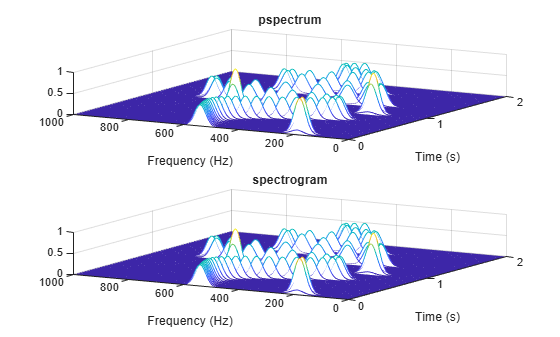
Generate a complex-valued signal with the same duration and sample rate. The signal is a chirp with sinusoidally varying frequency content and embedded in white noise. Compute the spectrogram of the signal and display it as a waterfall plot. For complex-valued signals, the spectrogram is two-sided by default.
x2 = exp(2j*pi*100*cos(2*pi*2*t)) + randn(size(t))/100;

[p,f,t] = pspectrum(x2,fs,"spectrogram");

waterfall(f,t,p')
xlabel("Frequency (Hz)")
ylabel("Time (seconds)")
wtf = gca;
wtf.XDir = "reverse";
view([30 45])

Generate a two-channel signal sampled at 100 Hz for 2 seconds.
The first channel consists of a 20 Hz tone and a 21 Hz tone. Both tones have unit amplitude.
The second channel also has two tones. One tone has unit amplitude and a frequency of 20 Hz. The other tone has an amplitude of 1/100 and a frequency of 30 Hz.
fs = 100;
t = (0:1/fs:2-1/fs)';

x = sin(2*pi*[20 20].*t) + [1 1/100].*sin(2*pi*[21 30].*t);
Embed the signal in white noise. Specify a signal-to-noise ratio of 40 dB. Plot the signals.
x = x + randn(size(x)).*std(x)/db2mag(40);

plot(t,x)

Compute the spectra of the two channels and display them.
pspectrum(x,t)

The default value for the spectral leakage, 0.5, corresponds to a resolution bandwidth of about 1.29 Hz. The two tones in the first channel are not resolved. The 30 Hz tone in the second channel is visible, despite being much weaker than the other one.
Increase the leakage to 0.85, equivalent to a resolution of about 0.74 Hz. The weak tone in the second channel is clearly visible.
pspectrum(x,t,Leakage=0.85)

Increase the leakage to the maximum value. The resolution bandwidth is approximately 0.5 Hz. The two tones in the first channel are resolved. The weak tone in the second channel is masked by the large window sidelobes.
pspectrum(x,t,Leakage=1)

Generate a signal that consists of a voltage-controlled oscillator and three Gaussian atoms. The signal is sampled at kHz for 2 seconds.
fs = 2000;
tx = 0:1/fs:2;
gaussFun = @(A,x,mu,f) exp(-(x-mu).^2/(2*0.03^2)).*sin(2*pi*f.*x)*A';
s = gaussFun([1 1 1],tx',[0.1 0.65 1],[2 6 2]*100)*1.5;
x = vco(chirp(tx+.1,0,tx(end),3).*exp(-2*(tx-1).^2),[0.1 0.4]*fs,fs);
x = s+x';
Short-Time Fourier Transforms
Use the pspectrum function to compute the STFT.
Divide the -sample signal into segments of length samples, corresponding to a time resolution of milliseconds.
Specify samples or 20% of overlap between adjoining segments.
Window each segment with a Kaiser window and specify a leakage .
M = 80;
L = 16;
lk = 0.7;

[S,F,T] = pspectrum(x,fs,"spectrogram", ...
    TimeResolution=M/fs,OverlapPercent=L/M*100, ...
    Leakage=lk);
Compare to the result obtained with the spectrogram function.
Specify the window length and overlap directly in samples.
pspectrumalways uses a Kaiser window as . The leakage and the shape factor of the window are related by .pspectrumalways uses points when computing the discrete Fourier transform. You can specify this number if you want to compute the transform over a two-sided or centered frequency range. However, for one-sided transforms, which are the default for real signals,spectrogramuses points. Alternatively, you can specify the vector of frequencies at which you want to compute the transform, as in this example.If a signal cannot be divided exactly into segments,
spectrogramtruncates the signal whereaspspectrumpads the signal with zeros to create an extra segment. To make the outputs equivalent, remove the final segment and the final element of the time vector.spectrogramreturns the STFT, whose magnitude squared is the spectrogram.pspectrumreturns the segment-by-segment power spectrum, which is already squared but is divided by a factor of before squaring.For one-sided transforms,
pspectrumadds an extra factor of 2 to the spectrogram.
g = kaiser(M,40*(1-lk));

k = (length(x)-L)/(M-L);
if k~=floor(k)
    S = S(:,1:floor(k));
    T = T(1:floor(k));
end

[s,f,t] = spectrogram(x/sum(g)*sqrt(2),g,L,F,fs);
Use the waterplot function to display the spectrograms computed by the two functions.
subplot(2,1,1)
waterplot(sqrt(S),F,T)
title("pspectrum")

subplot(2,1,2)
waterplot(s,f,t)
title("spectrogram")
maxd = max(max(abs(abs(s).^2-S)))
maxd =
2.4419e-08
Power Spectra and Convenience Plots
The spectrogram function has a fourth argument that corresponds to the segment-by-segment power spectrum or power spectral density. Similar to the output of pspectrum, the ps argument is already squared and includes the normalization factor . For one-sided spectrograms of real signals, you still have to include the extra factor of 2. Set the scaling argument of the function to "power".
[~,~,~,ps] = spectrogram(x*sqrt(2),g,L,F,fs,"power");

max(abs(S(:)-ps(:)))
ans = 2.4419e-08
When called with no output arguments, both pspectrum and spectrogram plot the spectrogram of the signal in decibels. Include the factor of 2 for one-sided spectrograms. Set the colormaps to be the same for both plots. Set the x-limits to the same values to make visible the extra segment at the end of the pspectrum plot. In the spectrogram plot, display the frequency on the y-axis.
subplot(2,1,1)
pspectrum(x,fs,"spectrogram", ...
    TimeResolution=M/fs,OverlapPercent=L/M*100, ...
    Leakage=lk)
title("pspectrum")
cc = clim;
xl = xlim;

subplot(2,1,2)
spectrogram(x*sqrt(2),g,L,F,fs,"power","yaxis")
title("spectrogram")
clim(cc)
xlim(xl)
function waterplot(s,f,t)
% Waterfall plot of spectrogram
    waterfall(f,t,abs(s)'.^2)
    set(gca,XDir="reverse",View=[30 50])
    xlabel("Frequency (Hz)")
    ylabel("Time (s)")
end
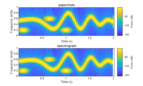
Visualize an interference narrowband signal embedded within a broadband signal.
Generate a chirp sampled at 1 kHz for 500 seconds. The frequency of the chirp increases from 180 Hz to 220 Hz during the measurement.
fs = 1000;
t = (0:1/fs:500)';

x = chirp(t,180,t(end),220) + 0.15*randn(size(t));
The signal also contains a 210 Hz sinusoid. The sinusoid has an amplitude of 0.05 and is present only for 1/6 of the total signal duration.
idx = floor(length(x)/6);
x(1:idx) = x(1:idx) + 0.05*cos(2*pi*t(1:idx)*210);
Compute the spectrogram of the signal. Restrict the frequency range from 100 Hz to 290 Hz. Specify a time resolution of 1 second. Both signal components are visible.
pspectrum(x,fs,"spectrogram", ...
    FrequencyLimits=[100 290],TimeResolution=1)

Compute the power spectrum of the signal. The weak sinusoid is obscured by the chirp.
pspectrum(x,fs,FrequencyLimits=[100 290])

Compute the persistence spectrum of the signal. Now both signal components are clearly visible.
pspectrum(x,fs,"persistence", ...
    FrequencyLimits=[100 290],TimeResolution=1)

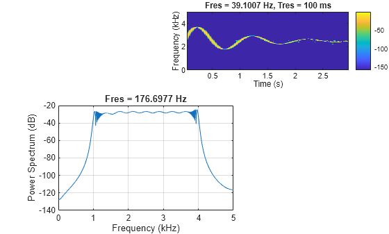
Generate a quadratic chirp sampled at 1 kHz for 2 seconds. The chirp has an initial frequency of 100 Hz that increases to 200 Hz at t = 1 second. Compute the spectrogram using the default settings of the pspectrum function. Use the waterfall function to plot the spectrogram.
fs = 1e3;
t = 0:1/fs:2;
y = chirp(t,100,1,200,"quadratic");

[sp,fp,tp] = pspectrum(y,fs,"spectrogram");

waterfall(fp,tp,sp')
set(gca,XDir="reverse",View=[60 60])
ylabel("Time (s)")
xlabel("Frequency (Hz)")

Compute and display the reassigned spectrogram.
[sr,fr,tr] = pspectrum(y,fs,"spectrogram",Reassign=true);

waterfall(fr,tr,sr')
set(gca,XDir="reverse",View=[60 60])
ylabel("Time (s)")
xlabel("Frequency (Hz)")

Recompute the spectrogram using a time resolution of 0.2 second. Visualize the result using the pspectrum function with no output arguments.
pspectrum(y,fs,"spectrogram",TimeResolution=0.2)
Compute the reassigned spectrogram using the same time resolution.
pspectrum(y,fs,"spectrogram",TimeResolution=0.2,Reassign=true)
Create a signal, sampled at 4 kHz, that resembles pressing all the keys of a digital telephone. Save the signal as a MATLAB® timetable.
fs = 4e3;
t = 0:1/fs:0.5-1/fs;

ver = [697 770 852 941];
hor = [1209 1336 1477];

tones = [];

for k = 1:length(ver)
    for l = 1:length(hor)
        tone = sum(sin(2*pi*[ver(k);hor(l)].*t))';
        tones = [tones;tone;zeros(size(tone))];
    end
end

% To hear, type soundsc(tones,fs)

S = timetable(seconds(0:length(tones)-1)'/fs,tones);
Compute the spectrogram of the signal. Specify a time resolution of 0.5 second and zero overlap between adjoining segments. Specify the leakage as 0.85, which is approximately equivalent to windowing the data with a Hann window.
pspectrum(S,"spectrogram", ...
    TimeResolution=0.5,OverlapPercent=0,Leakage=0.85)

The spectrogram shows that each key is pressed for half a second, with half-second silent pauses between keys. The first tone has a frequency content concentrated around 697 Hz and 1209 Hz, corresponding to the digit "1" in the DTMF standard.
Since R2026a
Plot the power spectrum, reassigned spectrogram, and persistence spectrum for four signals in the specified target axes and panel containers.
Create four oscillating signals with a sample rate of 10 kHz for three seconds.
Fs = 10e3;
t = 0:1/Fs:3;
x1 = vco(sawtooth(2*pi*t,0.5),[0.1 0.4]*Fs,Fs);
x2 = vco(sin(2*pi*t).*exp(-t),[0.1 0.4]*Fs,Fs) ...
    + 0.01*sin(2*pi*0.25*Fs*t);
x3 = exp(1j*pi*sin(4*t)*Fs/10);
x4 = chirp(t,Fs/10,t(end),Fs/2.5,"quadratic");
Plot Power Spectrum and Reassigned Spectrogram in Target Axes
Create two axes in the southwestern and northeastern corners of a new figure window.
fig = figure;
ax1 = axes(fig,Position=[0.15 0.1 0.45 0.45]);
ax2 = axes(fig,Position=[0.48 0.7 0.52 0.25]);
Plot the power spectrum and reassigned spectrogram of the signal x1 and x2 in the southwestern and northeastern axes of the figure, respectively. Set the time resolution to 0.1 seconds and specify a spectral leakage of 0.3.
pspectrum(x1,Fs,Parent=ax1)
pspectrum(x2,Fs,"spectrogram",Leakage=0.3, ...
    TimeResolution=0.1,Reassign=true,Parent=ax2)
Plot Power Spectrum in Target UI Axes
Create an axes in the northwestern corner of a new UI figure window.
uif = uifigure(Position=[100 100 720 540]);
ax3 = uiaxes(uif,Position=[5 305 300 200]);
Plot the power spectrum of the signal x3 on the figure axes. Set the frequency limits of the power spectrum to one fourth of the sample rate.
pspectrum(x3,Fs,FrequencyLimits=[-Fs/4 Fs/4],Parent=ax3)
title(ax3,"Power Spectrum in UI Axes")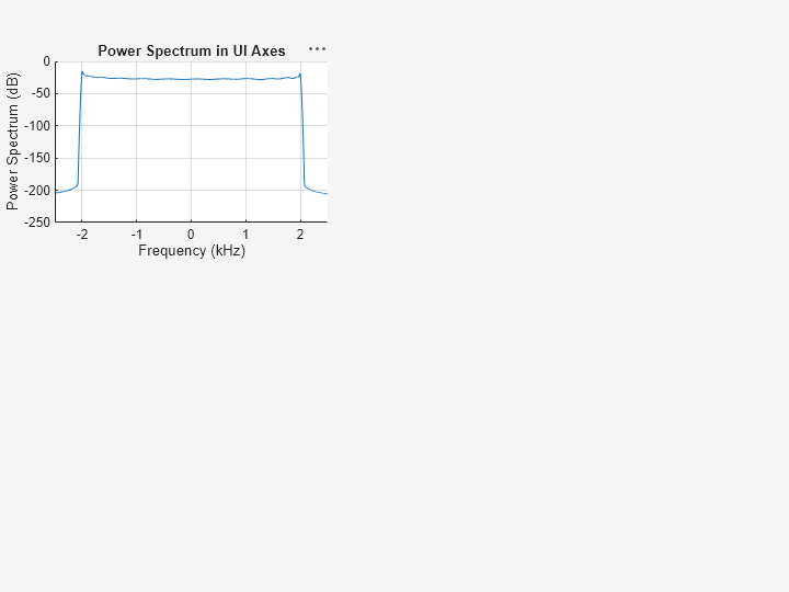
Plot Persistence Spectrum in Target Panel Container
Add a panel container in the southeastern corner of the UI figure window.
p = uipanel(uif,Position=[300 5 400 325], ...
    Title="Persistence Spectrum in Panel Container", ...
    BackgroundColor="white");
Plot the persistence spectrum of the signal x4 on the panel container.
pspectrum(x4,Fs,"persistence",Parent=p)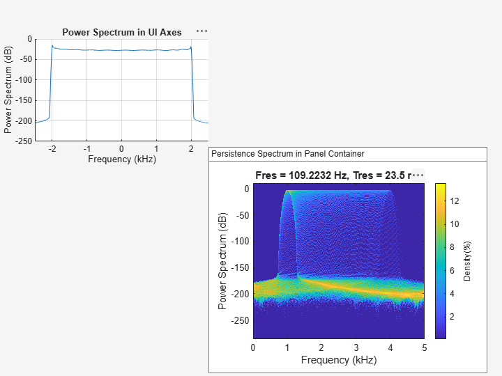
Input Arguments
Name-Value Arguments
Output Arguments
More About
To compute signal spectra, pspectrum finds a
compromise between the spectral resolution achievable with the entire length of the
signal and the performance limitations that result from computing large FFTs:
If possible, the function computes a single modified periodogram of the whole signal using a Kaiser window.
If it is not possible to compute a single modified periodogram in a reasonable amount of time, the function computes a Welch periodogram: It divides the signal into overlapping segments, windows each segment using a Kaiser window, and averages the periodograms of the segments.
Spectral Windowing
Any real-world signal is measurable only for a finite length of time. This fact introduces nonnegligible effects into Fourier analysis, which assumes that signals are either periodic or infinitely long. Spectral windowing, which assigns different weights to different signal samples, deals systematically with finite-size effects.
The simplest way to window a signal is to assume that it is identically zero outside of the measurement interval and that all samples are equally significant. This "rectangular window" has discontinuous jumps at both ends that result in spectral ringing. All other spectral windows taper at both ends to lessen this effect by assigning smaller weights to samples close to the signal edges.
The windowing process always involves a compromise between conflicting aims: improving resolution and decreasing leakage:
Resolution is the ability to know precisely how the signal energy is distributed in the frequency space. A spectrum analyzer with ideal resolution can distinguish two different tones (pure sinusoids) present in the signal, no matter how close in frequency. Quantitatively, this ability relates to the mainlobe width of the transform of the window.
Leakage is the fact that, in a finite signal, every frequency component projects energy content throughout the complete frequency span. The amount of leakage in a spectrum can be measured by the ability to detect a weak tone from noise in the presence of a neighboring strong tone. Quantitatively, this ability relates to the sidelobe level of the frequency transform of the window.
The spectrum is normalized so that a pure tone within that bandwidth, if perfectly centered, has the correct amplitude.
The better the resolution, the higher the leakage, and vice versa. At one end of the range, a rectangular window has the narrowest possible mainlobe and the highest sidelobes. This window can resolve closely spaced tones if they have similar energy content, but it fails to find the weaker one if they do not. At the other end, a window with high sidelobe suppression has a wide mainlobe in which close frequencies are smeared together.
pspectrum uses Kaiser windows to carry out windowing. For
Kaiser windows, the fraction of the signal energy captured by the mainlobe depends
most importantly on an adjustable shape factor,
β. pspectrum uses shape factors ranging
from β = 0, which corresponds to a rectangular window, to β = 40, where a wide mainlobe captures essentially all the spectral
energy representable in double precision. An intermediate value of β ≈ 6 approximates a Hann window quite closely. To control
β, use the Leakage name-value argument.
If you set Leakage to ℓ, then
ℓ and β are related by β = 40(1 – ℓ). See kaiser for more
details.
|
|
| 51-point Hann window and 51-point Kaiser window with β = 5.7 in the time domain | 51-point Hann window and 51-point Kaiser window with β = 5.7 in the frequency domain |


Parameter and Algorithm Selection
To compute signal spectra, pspectrum initially determines the
resolution bandwidth, which measures how close two tones
can be and still be resolved. The resolution bandwidth has a theoretical value of
tmax – tmin, the record length, is the time-domain duration of the selected signal region.
ENBW is the equivalent noise bandwidth of the spectral window. See
enbwfor more details.Use the
Leakagename-value argument to control the ENBW. The minimum value of the argument corresponds to a Kaiser window with β = 40. The maximum value corresponds to a Kaiser window with β = 0.
In practice, however, pspectrum might lower the resolution.
Lowering the resolution makes it possible to compute the spectrum in a reasonable
amount of time and to display it with a finite number of pixels. For these practical
reasons, the lowest resolution bandwidth pspectrum can use is
where fspan is the width of the frequency band specified using
FrequencyLimits. If FrequencyLimits is
not specified, then pspectrum uses the sample rate as fspan. RBWperformance cannot be adjusted.
To compute the spectrum of a signal, the function chooses the larger of the two values, called the target resolution bandwidth:
If the resolution bandwidth is RBWtheory, then
pspectrumcomputes a single modified periodogram for the whole signal. The function uses a Kaiser window with shape factor controlled by theLeakagename-value argument. Seeperiodogramfor more details.If the resolution bandwidth is RBWperformance, then
pspectrumcomputes a Welch periodogram for the signal. The function:Divides the signals into overlapping segments.
Windows each segment separately using a Kaiser window with the specified shape factor.
Averages the periodograms of all the segments.
Welch’s procedure is designed to reduce the variance of the spectrum estimate by averaging different “realizations” of the signals, given by the overlapping sections, and using the window to remove redundant data. See
pwelchfor more details.The length of each segment (or, equivalently, of the window) is computed using
where fNyquist is the Nyquist frequency. (If there is no aliasing, the Nyquist frequency is one-half the effective sample rate, defined as the inverse of the median of the differences between adjacent time points. The Nyquist range is [0, fNyquist] for real signals and [–fNyquist, fNyquist] for complex signals.)
The stride length is found by adjusting an initial estimate,
so that the first window starts exactly on the first sample of the first segment and the last window ends exactly on the last sample of the last segment.
The persistence spectrum is a time-frequency view that shows the percentage of the time that a given frequency is present in a signal. The persistence spectrum is a histogram in power-frequency space. The longer a particular frequency persists in a signal as the signal evolves, the higher its time percentage and thus the brighter or "hotter" its color in the display. Use the persistence spectrum to identify signals hidden in other signals.
To compute the persistence spectrum, pspectrum performs these steps:
Compute the spectrogram using the specified leakage, time resolution, and overlap. See Spectrogram Computation for more details.
Partition the power and frequency values into 2-D bins. (Use the
NumPowerBinsname-value argument to specify the number of power bins.)For each time value, compute a bivariate histogram of the logarithm of the power spectrum. For every power-frequency bin where there is signal energy at that instant, increase the corresponding matrix element by 1. Sum the histograms for all the time values.
Plot the accumulated histogram against the power and the frequency, with the color proportional to the logarithm of the histogram counts expressed as normalized percentages. To represent zero values, use one-half of the smallest possible magnitude.
| Power Spectra |
|
|
| Histograms |
|
|
| Accumulated Histogram |
|
|


References
[1] harris, fredric j. “On the Use of Windows for Harmonic Analysis with the Discrete Fourier Transform.” Proceedings of the IEEE®. Vol. 66, January 1978, pp. 51–83.
[2] Welch, Peter D. "The Use of Fast Fourier Transform for the Estimation of Power Spectra: A Method Based on Time Averaging Over Short, Modified Periodograms." IEEE Transactions on Audio and Electroacoustics. Vol. 15, June 1967, pp. 70–73.