pmtm

Multitaper power spectral density estimate

Syntax

pxx = pmtm(x)

pxx = pmtm(x,'Tapers',tapertype)

pxx = pmtm(x,nw)

pxx = pmtm(x,m,'Tapers','sine')

pxx = pmtm(___,nfft)

[pxx,w] = pmtm(___)

[pxx,f] = pmtm(___,fs)

[pxx,w] = pmtm(x,nw,w)

[pxx,w] = pmtm(x,m,'Tapers','sine',w)

[pxx,f] = pmtm(___,f,fs)

[___] = pmtm(___,freqrange)

[___,pxxc] = pmtm(___,'ConfidenceLevel',probability)

[___] = pmtm(___,'DropLastTaper',dropflag)

[___] = pmtm(___,method)

[___] = pmtm(x,e,v,___)

[___] = pmtm(x,dpss_params,___)

pmtm(___)

Description

pxx = pmtm(x) returns Thomson’s multitaper power spectral density (PSD) estimate, pxx, of the input signal x using Discrete Prolate Spheroidal (Slepian) Sequences as tapers.

pxx = pmtm(x,'Tapers',tapertype) specifies the type of tapers to use when computing the multitaper PSD estimate. You can specify the 'Tapers',tapertype name-value pair anywhere after x in the function call.

pxx = pmtm(x,nw) uses the time-halfbandwidth product nw to control the frequency resolution when computing a PSD estimate using Slepian tapers.

pxx = pmtm(x,m,'Tapers','sine') specifies the number of tapers or the averaging weights to apply when computing a PSD estimate using Sine Tapers.

pxx = pmtm(___,nfft) uses nfft discrete Fourier transform (DFT) points in combination with any of the previous syntaxes. If nfft is greater than the signal length, x is zero-padded to length nfft. If nfft is less than the signal length, the signal is wrapped modulo nfft.

[pxx,w] = pmtm(___) returns a vector with the normalized frequencies at which pxx is computed.

[pxx,f] = pmtm(___,fs) returns a frequency vector, f, in cycles per unit time. fs must follow x, nw (or m for sine tapers), and nfft in the function call. To input a sample rate and still use the default values of the preceding arguments, specify these arguments as empty, [].

[pxx,w] = pmtm(x,nw,w) returns the multitaper PSD estimate computed using Slepian sequences at the normalized frequencies specified in w. The vector w must contain at least two elements.

[pxx,w] = pmtm(x,m,'Tapers','sine',w) returns the multitaper PSD estimate computed using sine tapers at the normalized frequencies specified in w. The vector w must contain at least two elements.

[pxx,f] = pmtm(___,f,fs) computes the multitaper PSD estimate at the frequencies specified in f. The vector f must contain at least two elements in the same units as the sample rate fs.

[___] = pmtm(___,freqrange) returns the multitaper PSD estimate over the frequency range specified by freqrange.

[___,pxxc] = pmtm(___,'ConfidenceLevel',probability) returns the probability × 100% confidence intervals for the PSD estimate in pxxc.

[___] = pmtm(___,'DropLastTaper',dropflag) specifies whether pmtm drops the last Slepian taper when computing the multitaper PSD estimate.

[___] = pmtm(___,method) combines the individual tapered PSD estimates using the method specified in method. This syntax applies only to Slepian tapers.

[___] = pmtm(x,e,v,___) uses the Slepian tapers in e and the eigenvalues in v to compute the PSD. Use dpss to obtain e and v.

[___] = pmtm(x,dpss_params,___) uses the cell array dpss_params to pass input arguments to dpss. This syntax applies only to Slepian tapers.

pmtm(___) with no output arguments plots the multitaper PSD estimate in the current figure window.

Examples

Multitaper Estimate Using Default Inputs

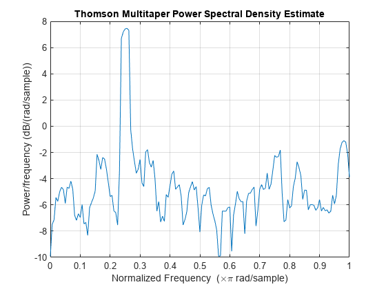
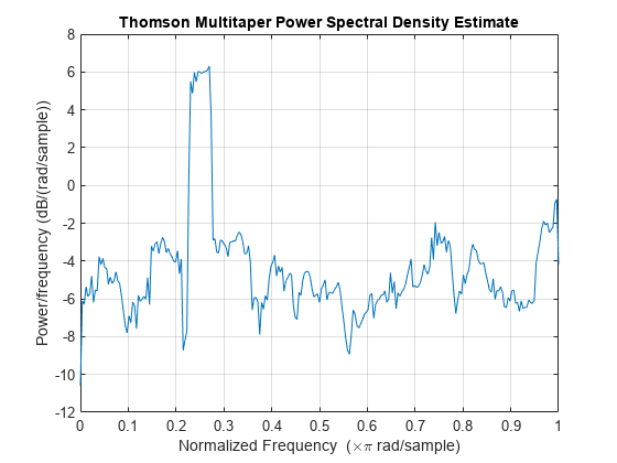
Obtain the multitaper PSD estimate of an input signal consisting of a discrete-time sinusoid with an angular frequency of $$\pi /4$$ rad/sample with additive N(0,1) white noise.

Create a sine wave with an angular frequency of $$\pi /4$$ rad/sample with additive N(0,1) white noise. The signal is 320 samples in length. Obtain the multitaper PSD estimate using the default time-halfbandwidth product of 4 and DFT length. The default number of DFT points is 512. Because the signal is real-valued, the PSD estimate is one-sided and there are 512/2+1 points in the PSD estimate.

n = 0:319;
x = cos(pi/4*n)+randn(size(n));
pxx = pmtm(x);

Plot the multitaper PSD estimate.

pmtm(x)

Sine and Slepian Tapers

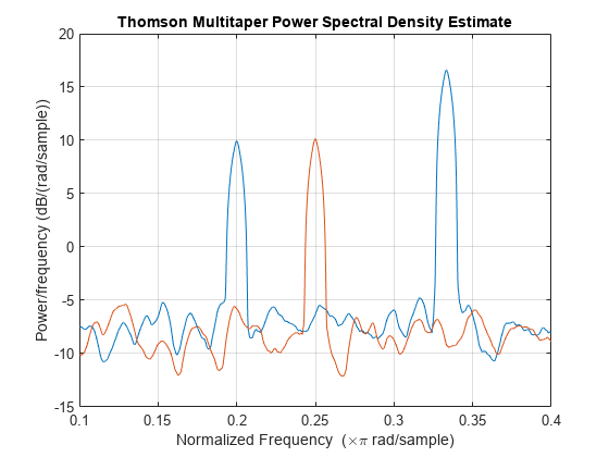
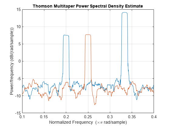
Generate 2048 samples of a two-channel signal embedded in additive N(0,1) white Gaussian noise.

• The first channel consists of two sinusoids with normalized frequencies of π/3 and π/5 rad/sample. The first sinusoid has twice the amplitude of the second.

• The second channel has a normalized frequency of π/4 rad/sample.

Use the multitaper method to estimate the PSD of the signal over a 1024-sample interval from 0.1π rad/sample to 0.4π rad/sample. Use 13 sine tapers weighted equally.

n = (0:2047)';

x = [sin(pi./[3 5].*n)*[2 1]' sin(pi/4*n)] + randn(length(n),2);

w = linspace(0.1,0.4,1024);

ntp = 13;
pmtm(x,ntp,'Tapers','sine',w*pi)

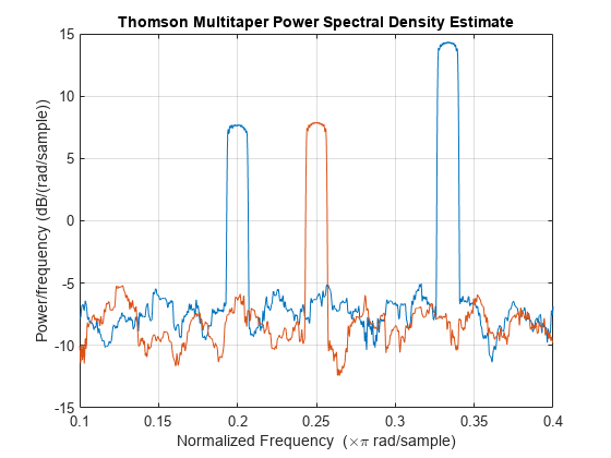
Repeat the computation, but now weight the 13 tapers in linear descending order. You can place the 'Tapers','sine' name-value pair anywhere after x in the function call.

pmtm(x,(ntp:-1:1)/sum(1:ntp),w*pi,'Tapers','sine')

Repeat the computation, but now use 13 Slepian tapers and specify a time-halfbandwidth product of 7.5.

nw = 7.5;

pmtm(x,{nw,ntp},w*pi)

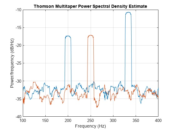
Repeat the computation, but now specify a sample rate of 2 kHz.

fs = 2e3;

pmtm(x,{nw,ntp},w*(fs/2),fs)

Specify Time-Halfbandwidth Product

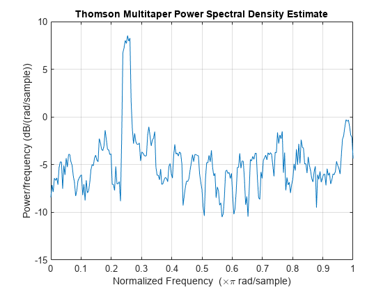
Obtain the multitaper PSD estimate with a specified time-halfbandwidth product.

Create a sine wave with an angular frequency of $$\pi /4$$ rad/sample with additive N(0,1) white noise. The signal is 320 samples in length. Obtain the multitaper PSD estimate with a time-halfbandwidth product of 2.5. The resolution bandwidth is $$[-2.5\pi /320,2.5\pi /320]$$ rad/sample. The default number of DFT points is 512. Because the signal is real-valued, the PSD estimate is one-sided and there are 512/2+1 points in the PSD estimate.

n = 0:319;
x = cos(pi/4*n)+randn(size(n));
pmtm(x,2.5)

DFT Length Equal to Signal Length

Obtain the multitaper PSD estimate of an input signal consisting of a discrete-time sinusoid with an angular frequency of $$\pi /4$$ rad/sample with additive N(0,1) white noise. Use a DFT length equal to the signal length.

Create a sine wave with an angular frequency of $$\pi /4$$ rad/sample with additive N(0,1) white noise. The signal is 320 samples in length. Obtain the multitaper PSD estimate with a time-halfbandwidth product of 3 and a DFT length equal to the signal length. Because the signal is real-valued, the one-sided PSD estimate is returned by default with a length equal to 320/2+1.

n = 0:319;
x = cos(pi/4*n)+randn(size(n));
pmtm(x,3,length(x))

Multitaper Estimate with Sample Rate

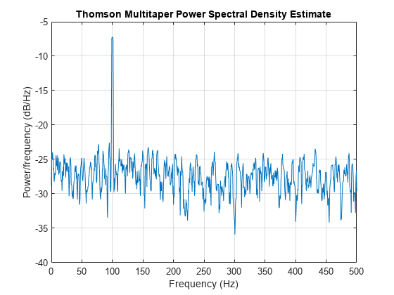
Obtain the multitaper PSD estimate of a signal sampled at 1 kHz. The signal is a 100 Hz sine wave in additive N(0,1) white noise. The signal duration is 2 s. Use a time-halfbandwidth product of 3 and DFT length equal to the signal length.

fs = 1000;
t = 0:1/fs:2-1/fs;
x = cos(2*pi*100*t)+randn(size(t));
[pxx,f] = pmtm(x,3,length(x),fs);

Plot the multitaper PSD estimate.

pmtm(x,3,length(x),fs)

Average Single-Taper Estimates with Unity Weights

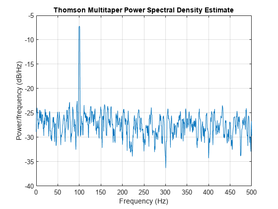
Obtain a multitaper PSD estimate where the individual tapered direct spectral estimates are given equal weight in the average.

Obtain the multitaper PSD estimate of a signal sampled at 1 kHz. The signal is a 100 Hz sine wave in additive N(0,1) white noise. The signal duration is 2 s. Use a time-halfbandwidth product of 3 and a DFT length equal to the signal length. Use the 'unity' option to give equal weight in the average to each of the individual tapered direct spectral estimates.

fs = 1000;
t = 0:1/fs:2-1/fs;
x = cos(2*pi*100*t)+randn(size(t));
[pxx,f] = pmtm(x,3,length(x),fs,'unity');

Plot the multitaper PSD estimate.

pmtm(x,3,length(x),fs,'unity')

DPSS Sequences and Their Frequency-Domain Concentrations

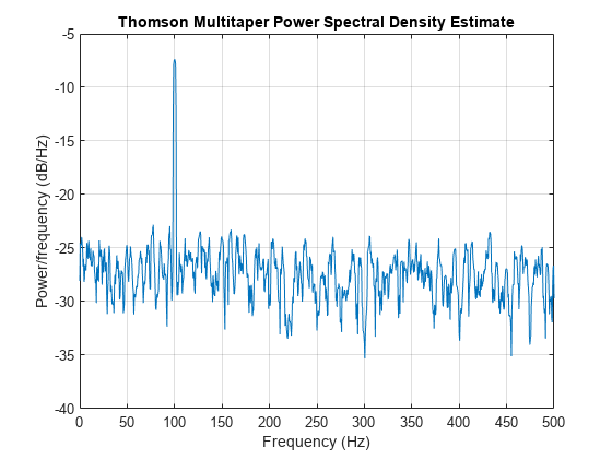
This example examines the frequency-domain concentrations of the DPSS sequences. The example produces a multitaper PSD estimate of an input signal by precomputing the Slepian sequences and selecting only those with more than 99% of their energy concentrated in the resolution bandwidth.

The signal is a 100 Hz sine wave in additive N(0,1) white noise. The signal duration is 2 seconds.

fs = 1000;
t = 0:1/fs:2-1/fs;
x = cos(2*pi*100*t)+randn(size(t));

Set the time-half-bandwidth product to 3.5. For the signal length of 2000 samples and a sampling interval of 0.001 seconds, this results in a resolution bandwidth of [–1.75,1.75] Hz. Calculate the first 10 Slepian sequences and examine their frequency concentrations in the specified resolution bandwidth.

[e,v] = dpss(length(x),3.5,10);
lv = length(v);

stem(1:lv,v,"filled")
ylim([0 1.2])
title("Proportion of Energy in [-w,w] of k-th Slepian Sequence")

Determine the number of Slepian sequences with energy concentrations greater than 99%. Using the selected DPSS sequences, obtain the multitaper PSD estimate. Set DropLastTaper to false to use all the selected tapers.

hold on
plot([1 lv],0.99*[1 1])
hold off

idx = find(v>0.99,1,'last')

idx = 
5

[pxx,f] = pmtm(x,e(:,1:idx),v(1:idx),length(x),fs,DropLastTaper=false);

Plot the multitaper PSD estimate.

pmtm(x,e(:,1:idx),v(1:idx),length(x),fs,DropLastTaper=false)

DC-Centered Multitaper PSD Estimate

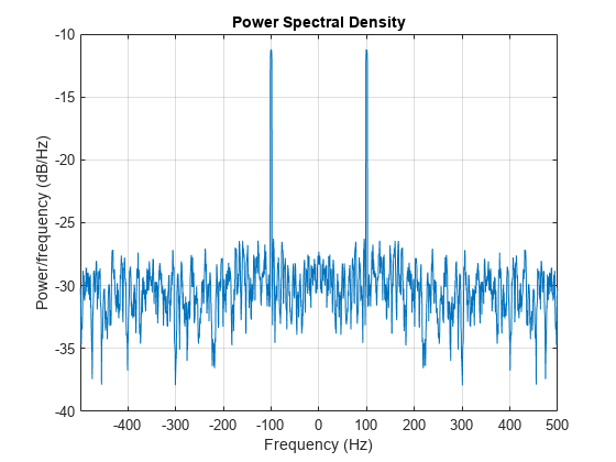
Obtain the multitaper PSD estimate of a 100 Hz sine wave in additive N(0,1) noise. The data are sampled at 1 kHz. Use the 'centered' option to obtain the DC-centered PSD.

fs = 1000;
t = 0:1/fs:2-1/fs;
x = cos(2*pi*100*t)+randn(size(t));
[pxx,f] = pmtm(x,3.5,length(x),fs,'centered');

Plot the DC-centered PSD estimate.

pmtm(x,3.5,length(x),fs,'centered')

Upper and Lower 95%-Confidence Bounds

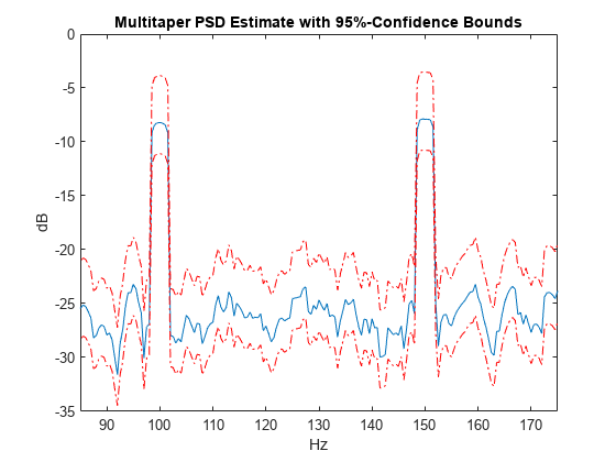
The following example illustrates the use of confidence bounds with the multitaper PSD estimate. While not a necessary condition for statistical significance, frequencies in the multitaper PSD estimate where the lower confidence bound exceeds the upper confidence bound for surrounding PSD estimates clearly indicate significant oscillations in the time series.

Create a signal consisting of the superposition of 100-Hz and 150-Hz sine waves in additive white N(0,1) noise. The amplitude of the two sine waves is 1. The sampling frequency is 1 kHz. The signal is 2 s in duration.

fs = 1000;
t = 0:1/fs:2-1/fs;
x = cos(2*pi*100*t)+cos(2*pi*150*t)+randn(size(t));

Obtain the multitaper PSD estimate with 95%-confidence bounds. Plot the PSD estimate along with the confidence interval and zoom in on the frequency region of interest near 100 and 150 Hz.

[pxx,f,pxxc] = pmtm(x,3.5,length(x),fs,'ConfidenceLevel',0.95);

plot(f,10*log10(pxx))
hold on
plot(f,10*log10(pxxc),'r-.')
xlim([85 175])
xlabel('Hz')
ylabel('dB')
title('Multitaper PSD Estimate with 95%-Confidence Bounds')

The lower confidence bound in the immediate vicinity of 100 and 150 Hz is significantly above the upper confidence bound outside the vicinity of 100 and 150 Hz.

Multitaper PSD Estimate of a Multichannel Signal

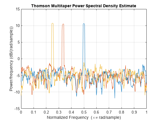
Generate 1024 samples of a multichannel signal consisting of three sinusoids in additive $$N(0,1)$$ white Gaussian noise. The sinusoids' frequencies are $$\pi /2$$, $$\pi /3$$, and $$\pi /4$$ rad/sample. Estimate the PSD of the signal using Thomson's multitaper method and plot it.

N = 1024;
n = 0:N-1;

w = pi./[2;3;4];
x = cos(w*n)' + randn(length(n),3);

pmtm(x)

Input Arguments

x — Input signal

vector | matrix

Input signal, specified as a row or column vector, or as a matrix. If x is a matrix, then its columns are treated as independent channels.

Example: cos(pi/4*(0:159))+randn(1,160) is a single-channel row-vector signal.

Example: cos(pi./[4;2]*(0:159))'+randn(160,2) is a two-channel signal.

Data Types: single | double
Complex Number Support: Yes

tapertype — Taper type

'slepian' (default) | 'sine'

Taper type, specified as 'slepian' or 'sine'.

• 'slepian' — Use Discrete Prolate Spheroidal (Slepian) Sequences as tapers.

• 'sine' — Use Sine Tapers.

You can specify the 'Tapers',tapertype name-value pair anywhere after x in the function call.

Data Types: char | string

nw — Time-halfbandwidth product

4 (default) | positive scalar

Time-halfbandwidth product, specified as a positive scalar. pmtm uses 2 × nw – 1 Slepian tapers in the PSD estimate. Typical choices for nw are 2, 5/2, 3, 7/2, or 4.

In multitaper spectral estimation, the user specifies the resolution bandwidth of the multitaper estimate [–W,W] where W = k/NΔt for some small k > 1. Equivalently, W is some small multiple of the frequency resolution of the DFT. The time-halfbandwidth product is the product of the resolution halfbandwidth and the number of samples in the input signal, N. The number of Slepian tapers whose Fourier transforms are well-concentrated in [–W,W] (eigenvalues close to unity) is 2NW – 1.

m — Sine taper number or averaging weights

7 (default) | integer scalar | vector

Sine taper number or averaging weights, specified as an integer scalar or a vector.

• If m is a scalar, it denotes the number of sine tapers used as data windows when computing the PSD estimate. The sine tapers are weighted uniformly.

• If m is a vector, it denotes the weights used to average the sine tapers when computing the PSD estimate. The length of m indicates the number of tapers to use. The elements of m must add to 1.

Data Types: single | double

nfft — Number of DFT points

max(256,2^nextpow2(length(x))) (default) | integer | []

Number of DFT points, specified as a positive integer. For a real-valued input signal, x, the PSD estimate, pxx has length (nfft/2 + 1) if nfft is even, and (nfft + 1)/2 if nfft is odd. For a complex-valued input signal,x, the PSD estimate always has length nfft. If nfft is specified as empty, the default nfft is used.

Data Types: single | double

fs — Sample rate

positive scalar

Sample rate, specified as a positive scalar. The sample rate is the number of samples per unit time. If the unit of time is seconds, then the sample rate has units of Hz.

w — Normalized frequencies

vector

Normalized frequencies, specified as a row or column vector with at least two elements. Normalized frequencies are in rad/sample.

Example: w = [pi/4 pi/2]

Data Types: double | single

f — Frequencies

vector

Frequencies, specified as a row or column vector with at least two elements. The frequencies are in cycles per unit time. The unit time is specified by the sample rate, fs. If fs has units of samples/second, then f has units of Hz.

Example: fs = 1000; f = [100 200]

Data Types: double | single

dropflag — Flag indicating whether to drop or keep the last DPSS sequence

true (default) | false

Flag indicating whether to drop or keep the last DPSS sequence, specified as a logical. The default is true and pmtm drops the last taper. In a multitaper estimate, the first 2NW – 1 DPSS sequences have eigenvalues close to unity. If you use less than 2NW – 1 sequences, it is likely that all the tapers have eigenvalues close to 1 and you can specify dropflag as false to keep the last taper.

method — Weights on individual tapered PSD estimates

'adapt' (default) | 'eigen' | 'unity'

Weights on individual tapered PSD estimates, specified as one of 'adapt', 'eigen', or 'unity'. The default is Thomson’s adaptive frequency-dependent weights, 'adapt'. The calculation of these weights is detailed on pp. 368–370 in [2]. The 'eigen' method weights each tapered PSD estimate by the eigenvalue (frequency concentration) of the corresponding Slepian taper. The 'unity' method weights each tapered PSD estimate equally.

e — DPSS (Slepian) sequences

matrix

DPSS (Slepian) sequences, specified as a matrix. If x has length N, then e has N rows. The matrix e is an output of dpss.

v — Eigenvalues for DPSS (Slepian) sequences

vector

Eigenvalues for DPSS (Slepian) sequences, specified as a column vector. The eigenvalues for the DPSS sequences indicate the proportion of the sequence energy concentrated in the resolution bandwidth, [–W, W]. The eigenvalues range lie in the interval (0, 1) and generally the first 2NW – 1 eigenvalues are close to 1 and then decrease toward 0. The vector v is an output of dpss.

dpss_params — Input arguments for dpss

cell array

Input arguments for dpss, specified as a cell array. The first input argument to dpss is the length of the DPSS sequences and is omitted from dpss_params because it is obtained from the length of x.

Example: pmtm(randn(1000,1),{2.5,3}) computes the PSD of a random sequence using the first 3 Slepian sequences with time-halfbandwidth product 2.5.

freqrange — Frequency range for PSD estimate

'onesided' | 'twosided' | 'centered'

Frequency range for the PSD estimate, specified as a one of 'onesided', 'twosided', or 'centered'. The default is 'onesided' for real-valued signals and 'twosided' for complex-valued signals. The frequency ranges corresponding to each option are

• 'onesided' — returns the one-sided PSD estimate of a real-valued input signal, x. If nfft is even, pxx has length nfft/2 + 1 and is computed over the interval [0,π] rad/sample. If nfft is odd, the length of pxx is (nfft + 1)/2 and the interval is [0,π) rad/sample. When fs is optionally specified, the corresponding intervals are [0,fs/2] cycles/unit time and [0,fs/2) cycles/unit time for even and odd length nfft respectively.

  The function multiplies the power by 2 at all frequencies except 0 and the Nyquist frequency to conserve the total power.

• 'twosided' — returns the two-sided PSD estimate for either the real-valued or complex-valued input, x. In this case, pxx has length nfft and is computed over the interval [0,2π) rad/sample. When fs is optionally specified, the interval is [0,fs) cycles/unit time.

• 'centered' — returns the centered two-sided PSD estimate for either the real-valued or complex-valued input, x. In this case, pxx has length nfft and is computed over the interval (–π,π] rad/sample for even length nfft and (–π,π) rad/sample for odd length nfft. When fs is optionally specified, the corresponding intervals are (–fs/2, fs/2] cycles/unit time and (–fs/2, fs/2) cycles/unit time for even and odd length nfft respectively.

Data Types: char | string

probability — Confidence interval for PSD estimate

0.95 (default) | scalar in the range (0,1)

Coverage probability for the true PSD, specified as a scalar in the range (0,1). The output, pxxc, contains the lower and upper bounds of the probability × 100% interval estimate for the true PSD.

Output Arguments

pxx — PSD estimate

vector | matrix

PSD estimate, returned as a real-valued, nonnegative column vector or matrix. Each column of pxx is the PSD estimate of the corresponding column of x. The units of the PSD estimate are in squared magnitude units of the time series data per unit frequency. For example, if the input data is in volts, the PSD estimate is in units of squared volts per unit frequency. For a time series in volts, if you assume a resistance of 1 Ω and specify the sample rate in hertz, the PSD estimate is in watts per hertz.

w — Normalized frequencies

vector

Normalized frequencies, returned as a real-valued column vector. If pxx is a one-sided PSD estimate, w spans the interval [0,π] if nfft is even and [0,π) if nfft is odd. If pxx is a two-sided PSD estimate, w spans the interval [0,2π). For a DC-centered PSD estimate, w spans the interval (–π,π] for even nfft and (–π,π) for odd nfft.

f — Cyclical frequencies

vector

Cyclical frequencies, returned as a real-valued column vector. For a one-sided PSD estimate, f spans the interval [0,fs/2] when nfft is even and [0,fs/2) when nfft is odd. For a two-sided PSD estimate, f spans the interval [0,fs). For a DC-centered PSD estimate, f spans the interval (–fs/2, fs/2] cycles/unit time for even length nfft and (–fs/2, fs/2) cycles/unit time for odd length nfft.

pxxc — Confidence bounds

matrix

Confidence bounds, returned as a matrix with real-valued elements. The row size of the matrix is equal to the length of the PSD estimate, pxx. pxxc has twice as many columns as pxx. Odd-numbered columns contain the lower bounds of the confidence intervals, and even-numbered columns contain the upper bounds. Thus, pxxc(m,2*n-1) is the lower confidence bound and pxxc(m,2*n) is the upper confidence bound corresponding to the estimate pxx(m,n). The coverage probability of the confidence intervals is determined by the value of the probability input.

Data Types: single | double

More About

Thomson's Multitaper Spectral Estimation

The periodogram is not a consistent estimator of the true power spectral density (PSD) of a wide-sense stationary process. To reduce the variability in the periodogram — and thus produce a consistent estimate of the PSD — the multitaper method averages modified periodograms obtained using a family of mutually orthogonal windows or tapers. In addition to mutual orthogonality, the tapers also have optimal time-frequency concentration properties. Both the orthogonality and time-frequency concentration of the tapers are critical to the success of the multitaper technique. See Discrete Prolate Spheroidal (Slepian) Sequences for a brief description of the Slepian sequences used in Thomson’s multitaper method.

The multitaper method uses K modified periodograms, each one obtained using a different Slepian sequence as the window. Let

$$S_k(f)=\Delta t{\left|{\displaystyle \sum _{n=0}^{N-1}{g}_k\left(n\right)}x\left(n\right)e^{-j2\pi fn\Delta t}\right|}^2$$

denote the modified periodogram obtained with the kth Slepian sequence, g_k(n). In its simplest form, the multitaper method simply averages the K modified periodograms to produce the multitaper PSD estimate:

$$S^{(\text{MT})}(f)=\frac{1}{K}{\displaystyle \sum _{k=0}^{K-1}{S}_k}(f).$$

Thomson's multitaper approach, introduced in [4], resembles Welch’s overlapped segment averaging method, in that both average over approximately uncorrelated estimates of the PSD. However, the two approaches differ in how they produce these uncorrelated PSD estimates. The multitaper method uses the entire signal in each modified periodogram. The orthogonality of the Slepian tapers decorrelates the different modified periodograms. Welch’s approach uses segments of the signal in each modified periodogram, and the segmenting decorrelates the different modified periodograms.

The equation for S^(MT)(f) corresponds to the 'unity' option in pmtm. However, as explained in Discrete Prolate Spheroidal (Slepian) Sequences, the Slepian sequences do not possess equal energy concentration in the frequency band of interest. The higher the order of the Slepian sequence, the less concentrated the sequence energy is in the band [–W,W] with the concentration given by the eigenvalue. Consequently, it can be beneficial to use the eigenvalues to weight the K modified periodograms prior to averaging. This corresponds to the 'eigen' option in pmtm.

Using the sequence eigenvalues to produce a weighted average of modified periodograms accounts for the frequency concentration properties of the Slepian sequences. However, it does not account for the interaction between the power spectral density of the random process and the frequency concentration of the Slepian sequences. Specifically, frequency regions where the random process has little power are less reliably estimated in the modified periodograms using higher-order Slepian sequences. This argues for a frequency-dependent adaptive process, which accounts not only for the frequency concentration of the Slepian sequence but also for the power distribution in the time series. This adaptive weighting corresponds to the 'adapt' option in pmtm and is the default for computing the multitaper estimate.

Discrete Prolate Spheroidal (Slepian) Sequences

The derivation of the Slepian sequences proceeds from the discrete-time/continuous-frequency concentration problem. For all ℓ² sequences index-limited to 0, 1, …, N – 1, the problem seeks the sequence having the maximal concentration of its energy in a frequency band [–W, W] with |W| < 1/2Δt.

This amounts to finding the eigenvalues and corresponding eigenvectors of an N-by-N self-adjoint positive semidefinite operator. Therefore, the eigenvalues are real and nonnegative and eigenvectors corresponding to distinct eigenvalues are mutually orthogonal. In this particular problem, the eigenvalues are bounded by 1 and the eigenvalue is the measure of the sequence’s energy concentration in the frequency interval [–W, W].

The eigenvalue problem is given by

$${\displaystyle \sum _{m=0}^{N-1}\frac{\sin \left(2\pi W\left(n-m\right)\right)}{\pi \left(n-m\right)}}{g}_k\left(m\right)={\lambda }_k\left(N,W\right)g_k\left(n\right),n,k=0,1,2,\dots ,N-1.$$

The zeroth-order DPSS sequence, g₀, is the eigenvector corresponding to the largest eigenvalue. The first-order DPSS sequence, g₁, is the eigenvector corresponding to the next largest eigenvalue and is orthogonal to the zeroth-order sequence. The second-order DPSS sequence, g₂, is the eigenvector corresponding to the third-largest eigenvalue and is orthogonal to the two lower-order DPSS sequences. Because the operator is N-by-N, there are N eigenvectors. However, for a given sequence length N and a specified bandwidth [–W, W], there are approximately 2NW – 1 DPSS sequences with eigenvalues very close to unity. Use nw to specify NW.

Sine Tapers

Sine tapers, an alternative to Slepian sequences proposed in [3], are defined by

$$g_k(n)=\sqrt{\frac{2}{N+1}}\sin \frac{\pi kn}{N+1},n,k=1,2,\dots ,N.$$

Unlike Slepian sequences, sine tapers can be computed directly, with no need to set up and solve an eigenvalue equation. This makes sine tapers much faster to compute. Sine tapers have a spectral concentration close to that of Slepian sequences but do not need additional parameters to specify the spectral bandwidth. The bandwidth of the PSD estimate computed using sine tapers can be adjusted locally by changing the number of tapers using m.

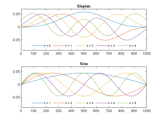
Compare Slepian and Sine Tapers

Generate the first five Slepian tapers corresponding to a time-halfbandwidth product of 3. Specify a taper length of 1000.

N = 1000;
nw = 3;
ns = 2*(nw)-1;

tprs = dpss(N,nw,ns);
lbs = "Slepian";

Generate the first five sine tapers.

n = 1:N;
k = 1:ns;

tprs(:,:,2) = sqrt(2/(N+1))*sin(pi*n'*k/(N+1));
lbs(2) = "Sine";

Plot the two sets of tapers.

for kj = 1:2
    subplot(2,1,kj)
    plot(tprs(:,:,kj))
    title(lbs(kj))
    legend(append('k = ',string(k+kj-2)), ...
        'Orientation','horizontal','Location','south')
    legend('boxoff')
    ylim([-0.09 0.07])
end

References

[1] McCoy, Emma J., Andrew T. Walden, and Donald B. Percival. "Multitaper Spectral Estimation of Power Law Processes." IEEE^® Transactions on Signal Processing 46, no. 3 (March 1998): 655–68. https://doi.org/10.1109/78.661333.

[2] Percival, Donald B., and Andrew T. Walden. Spectral Analysis for Physical Applications: Multitaper and Conventional Univariate Techniques. Cambridge; New York, NY, USA: Cambridge University Press, 1993.

[3] Riedel, Kurt S., and Alexander Sidorenko. “Minimum Bias Multiple Taper Spectral Estimation.” IEEE Transactions on Signal Processing 43, no. 1 (January 1995): 188–95. https://doi.org/10.1109/78.365298.

[4] Thomson, David J. "Spectrum estimation and harmonic analysis." Proceedings of the IEEE 70, no. 9 (1982): 1055–96. https://doi.org/10.1109/PROC.1982.12433.

Extended Capabilities

C/C++ Code Generation

Generate C and C++ code using MATLAB® Coder™.

Usage notes and limitations:

• Input arguments nfft and nw must be scalars during code generation.

• If nfft and nw are variable-sized, then the function considers nfft as the frequency vector f and nw as the matrix of Slepian tapers e.

Version History

Introduced before R2006a

R2023b: Generate C and C++ code

Generate C and C++ code for the pmtm function. You must have MATLAB^® Coder™ to use this functionality.