periodogram

Periodogram power spectral density estimate

Syntax

pxx = periodogram(x)

[pxx,f] = periodogram(x,win,freqSpec)

[pxx,f] = periodogram(x,win,freqSpec,Fs)

[pxx,f] = periodogram(___,freqRange,spectrumType)

[rpxx,f,pxx,fc] = periodogram(___,"reassigned")

[pxx,f,pxxc] = periodogram(___,ConfidenceLevel=p)

[___] = periodogram(___,Parent=h)

periodogram(___)

Description

pxx = periodogram(x) returns the periodogram power spectral density (PSD) estimate of the signal x. The function treats the column of x as independent channels.

[pxx,f] = periodogram(x,win,freqSpec) returns the periodogram PSD estimate of the signal x and the frequencies f (rad/sample), where the periodogram function:

• Uses win to divide the signal into segments and windows them.

• Computes the discrete Fourier transform (DFT) over the number of DFT points or at the frequencies specified in freqSpec.

To use default values for any of these input arguments, specify them as empty, [].

[pxx,f] = periodogram(x,win,freqSpec,Fs) specifies the sample rate Fs and returns the cyclical frequencies f in Hz.

[pxx,f] = periodogram(___,freqRange,spectrumType) also specifies the frequency range and spectrum type for any of the previous syntaxes. You can specify either or both of these input arguments.

[rpxx,f,pxx,fc] = periodogram(___,"reassigned") reassigns each PSD estimate or power spectrum estimate to the location of its center of energy. The vector rpxx contains the sum of the estimates reassigned to each element of f. This syntax also returns the center-of-energy frequencies, fc.

If your signal contains well-localized spectral components, then the "reassigned" argument generates a sharper periodogram.

[pxx,f,pxxc] = periodogram(___,ConfidenceLevel=p) returns the p × 100% confidence intervals for the PSD estimate in pxxc.

If you use the "reassigned" option, then you cannot specify a confidence interval.

[___] = periodogram(___,Parent=h) plots the periodogram PSD estimate or power spectrum in the target parent container h.

periodogram(___) with no output arguments plots the periodogram PSD estimate or power spectrum in the current figure window.

Examples

Periodogram Using Default Inputs

Obtain the periodogram of an input signal consisting of a discrete-time sinusoid with an angular frequency of $$\pi /4$$ rad/sample with additive $$N(0,1)$$ white noise.

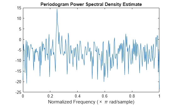
Create a sine wave with an angular frequency of $$\pi /4$$ rad/sample with additive $$N(0,1)$$ white noise. The signal is 320 samples in length. Obtain the periodogram using the default rectangular window and DFT length. The DFT length is the next power of two greater than the signal length, or 512 points. Because the signal is real-valued and has even length, the periodogram is one-sided and there are 512/2+1 points.

n = 0:319;
x = cos(pi/4*n) + randn(size(n));
[pxx,w] = periodogram(x);
plot(w/pi,pow2db(pxx))
xlabel("Normalized Frequency (\times \pi rad/sample)")
title("Periodogram Power Spectral Density Estimate")

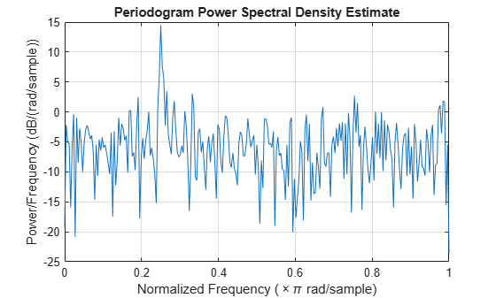
Repeat the plot using periodogram with no outputs.

periodogram(x)

Modified Periodogram with Hamming Window

Obtain the modified periodogram of an input signal consisting of a discrete-time sinusoid with an angular frequency of $$\pi /4$$ radians/sample with additive $$N(0,1)$$ white noise.

Create a sine wave with an angular frequency of $$\pi /4$$ radians/sample with additive $$N(0,1)$$ white noise. The signal is 320 samples in length. Obtain the modified periodogram using a Hamming window and default DFT length. The DFT length is the next power of two greater than the signal length, or 512 points. Because the signal is real-valued and has even length, the periodogram is one-sided and there are 512/2+1 points.

n = 0:319;
x = cos(pi/4*n) + randn(size(n));
periodogram(x,hamming(length(x)))

DFT Length Equal to Signal Length

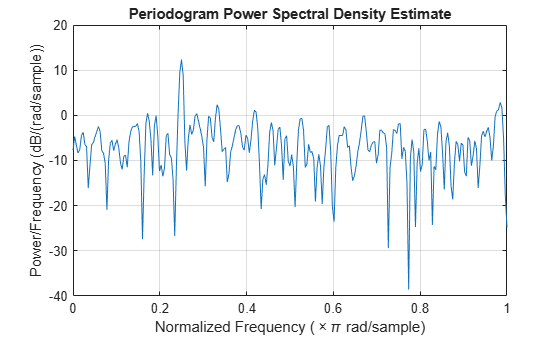
Obtain the periodogram of an input signal consisting of a discrete-time sinusoid with an angular frequency of $$\pi /4$$ radians/sample with additive $$N(0,1)$$ white noise. Use a DFT length equal to the signal length.

Create a sine wave with an angular frequency of $$\pi /4$$ radians/sample with additive $$N(0,1)$$ white noise. The signal is 320 samples in length. Obtain the periodogram using the default rectangular window and DFT length equal to the signal length. Because the signal is real-valued, the one-sided periodogram is returned by default with a length equal to 320/2+1.

rng("default")
n = 0:319;
x = cos(pi/4*n) + randn(size(n));
nfft = length(x);
periodogram(x,[],nfft)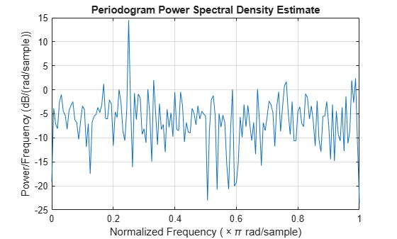

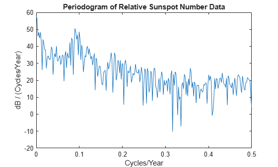
Periodogram of Relative Sunspot Numbers

Obtain the periodogram of the Wolf (relative sunspot) number data sampled yearly between 1700 and 1987.

Load the relative sunspot number data. Obtain the periodogram using the default rectangular window and number of DFT points (512 in this example). The sample rate for these data is 1 sample/year.

load sunspot.dat
relNums=sunspot(:,2);

[pxx,f] = periodogram(relNums,[],[],1);

Plot the periodogram. There is a peak in the periodogram at approximately 0.1 cycles/year, which indicates a period of approximately 10 years.

plot(f,pow2db(pxx))
xlabel("Cycles/Year")
ylabel("dB / (Cycles/Year)")
title("Periodogram of Relative Sunspot Number Data")

Periodogram at a Given Set of Normalized Frequencies

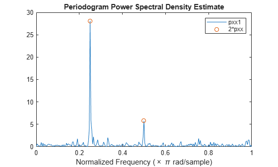
Obtain the periodogram of an input signal consisting of two discrete-time sinusoids with an angular frequencies of $$\pi /4$$ and $$\pi /2$$ rad/sample in additive $$N(0,1)$$ white noise. Obtain the two-sided periodogram estimates at $$\pi /4$$ and $$\pi /2$$ rad/sample.

n = 0:319;
x = cos(pi/4*n) + 0.5*sin(pi/2*n) + randn(size(n));

[pxx,w] = periodogram(x,[],[pi/4 pi/2]);
pxx

pxx = 1×2

   14.0589    2.8872

[pxx1,w1] = periodogram(x);

Compare the result to the one-sided periodogram. The periodogram values obtained are 1/2 the values in the one-sided periodogram. When you evaluate the periodogram at a specific set of frequencies, the output is a two-sided estimate.

plot(w1/pi,pxx1,w/pi,2*pxx,"o")
legend("pxx1","2*pxx")
xlabel("Normalized Frequency (\times \pi rad/sample)")
title("Periodogram Power Spectral Density Estimate")

Periodogram at a Given Set of Cyclical Frequencies

Create a signal consisting of two sine waves with frequencies of 100 and 200 Hz in N(0,1) white additive noise. The sample rate is 1 kHz. Obtain the two-sided periodogram at 100 and 200 Hz.

rng("default")
Fs = 1000;
t = 0:0.001:1-0.001;
x = cos(2*pi*100*t) + sin(2*pi*200*t) + randn(size(t));

freq = [100 200];
pxx = periodogram(x,[],freq,Fs)

pxx = 1×2

    0.2647    0.2313

Upper and Lower 95%-Confidence Bounds

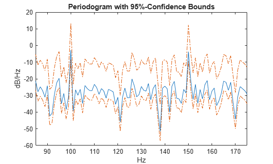
This example illustrates the use of confidence bounds with the periodogram. While not a necessary condition for statistical significance, frequencies in the periodogram where the lower confidence bound exceeds the upper confidence bound for surrounding PSD estimates clearly indicate significant oscillations in the time series.

Create a signal consisting of the superposition of 100 Hz and 150 Hz sine waves in additive white N(0,1) noise. The amplitude of the two sine waves is 1. The sample rate is 1 kHz.

rng("default")
Fs = 1000;
t = 0:1/Fs:1-1/Fs;
x = cos(2*pi*100*t) + sin(2*pi*150*t) + randn(size(t));

Obtain the periodogram PSD estimate with 95%-confidence bounds.

L = length(x);
[pxx,f,pxxc] = periodogram(x,rectwin(L),L,Fs,ConfidenceLevel=0.95);

Plot the periodogram along with the confidence interval and zoom in on the frequency region of interest near 100 and 150 Hz. The lower confidence bound in the immediate vicinity of 100 and 150 Hz is significantly above the upper confidence bound outside the vicinity of 100 and 150 Hz.

plot(f,pow2db(pxx))
hold on
plot(f,pow2db(pxxc),"-.",Color=[0.866 0.329 0])

xlim([85 175])
xlabel("Hz")
ylabel("dB/Hz")
title("Periodogram with 95%-Confidence Bounds")

DC-Centered Periodogram

Obtain the periodogram of a 100 Hz sine wave in additive $$N(0,1)$$ noise. The sample rate is 1 kHz. Use the "centered" option to obtain the DC-centered periodogram and plot the result.

fs = 1000;
t = 0:0.001:1-0.001;
x = cos(2*pi*100*t)+randn(size(t));
periodogram(x,[],length(x),fs,"centered")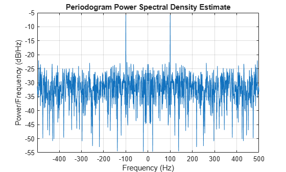

Reassigned Periodogram

Generate a signal that consists of a 200 Hz sinusoid embedded in white Gaussian noise. The signal is sampled at 1 kHz for 1 second. The noise has a variance of 0.01². Reset the random number generator for reproducible results.

rng("default")

Fs = 1000;
t = 0:1/Fs:1-1/Fs;
N = length(t);
x = sin(2*pi*t*200) + 0.01*randn(size(t));

Use the FFT to compute the power spectrum of the signal, normalized by the signal length. The sinusoid is in-bin, so all the power is concentrated in a single frequency sample. Plot the one-sided spectrum. Zoom in to the vicinity of the peak.

q = fft(x,N);
ff = 0:Fs/N:Fs-Fs/N;

ffts = q*q'/N^2

ffts = 
0.4997

ff = ff(1:floor(N/2)+1);
q = q(1:floor(N/2)+1);

stem(ff,abs(q)/N,"*")
axis([190 210 0 0.55])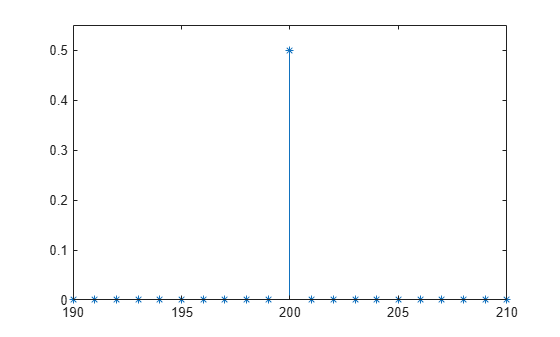

Use periodogram to compute the power spectrum of the signal. Specify a Hann window and an FFT length of 1024. Find the percentage difference between the estimated power at 200 Hz and the actual value.

wind = hann(N);

[pun,fr] = periodogram(x,wind,1024,Fs,"power");

hold on
stem(fr,pun)

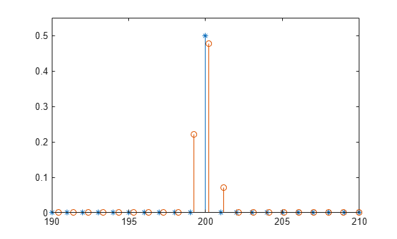
periodogErr = abs(max(pun)-ffts)/ffts*100

periodogErr = 
4.7349

Recompute the power spectrum, but this time use reassignment. Plot the new estimate and compare its maximum with the FFT value.

[pre,ft,pxx,fx] = periodogram(x,wind,1024,Fs,"power","reassigned");

stem(fx,pre)
hold off
legend(["Original" "Periodogram" "Reassigned"])

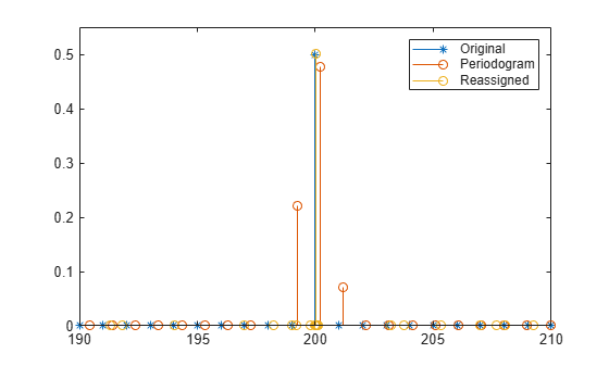
reassignErr = abs(max(pre)-ffts)/ffts*100

reassignErr = 
0.0779

Power Estimate of Sinusoid

Estimate the power of sinusoid at a specific frequency using the "power" option.

Create a 100 Hz sinusoid one second in duration sampled at 1 kHz. The amplitude of the sine wave is 1.8, which equates to a power of 1.8²/2 = 1.62. Estimate the power using the "power" option.

fs = 1000;
t = 0:1/fs:1-1/fs;
x = 1.8*cos(2*pi*100*t);
[pxx,f] = periodogram(x,hamming(length(x)),length(x),fs,"power");
[pwrest,idx] = max(pxx);
fprintf("The maximum power occurs at %3.1f Hz\n",f(idx))

The maximum power occurs at 100.0 Hz

fprintf("The power estimate is %2.2f\n",pwrest)

The power estimate is 1.62

Periodogram PSD Estimate of a Multichannel Signal

Generate 1024 samples of a multichannel signal consisting of three sinusoids in additive $$N(0,1)$$ white Gaussian noise. The sinusoids frequencies are $$\pi /2$$, $$\pi /3$$, and $$\pi /4$$ rad/sample. Estimate the PSD of the signal using the periodogram and plot it.

rng("default")
N = 1024;
n = 0:N-1;

w = pi./[2;3;4];
x = cos(w*n)' + randn(length(n),3);

periodogram(x)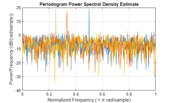

Compute Modified Periodogram Using Generated C Code

Examine the function myPeriodogram.m that returns the Modified Periodogram power spectral density (PSD) estimate of an input signal using a window. The function specifies a number of discrete Fourier transform points equal to the length of the input signal.

type myPeriodogram

function [pxx,f] = myPeriodogram(inputData,window) %#codegen
    nfft = length(inputData);
    [pxx,f] = periodogram(inputData,window,nfft);
end

Use codegen (MATLAB Coder) to generate a MEX function.

• The %#codegen directive in the function indicates that the MATLAB® code is intended for code generation.

• The -args option specifies example arguments that define the size, class, and complexity of the inputs to the MEX-file. For this example, specify inputData as a 1024-by-1 double precision random vector and window as a Hamming window of length 1024. In subsequent calls to the MEX function, use 1024-sample input signals and windows.

• To set a different name for the MEX function, use the -o option.

• To generate a code generation report, add the -report option at the end of the codegen command.

codegen myPeriodogram -args {randn(1024,1),hamming(1024)}

Code generation successful.

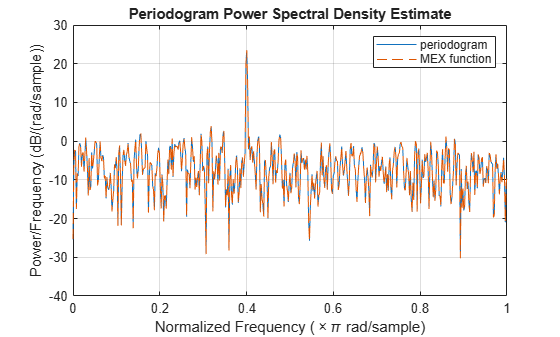
Compute the PSD estimate of a 1024-sample noisy sinusoid using the periodogram function and the generated MEX function. Specify a sinusoid normalized frequency of $2\pi /5$ rad/sample and a Hann window. Plot the two estimates to verify that they coincide.

N = 1024;
x = 2*cos(2*pi/5*(0:N-1)') + randn(N,1);
periodogram(x,hann(N))
[pxMex,fMex] = myPeriodogram_mex(x,hann(N));
hold on
plot(fMex/pi,pow2db(pxMex),"--")
hold off
grid on
legend(["periodogram" "MEX function"])

Plot Periodograms in Target Axes and Panel Container

Since R2026a

Plot the periodogram power spectral density (PSD) estimate and periodogram power spectrum for four signals in the specified target axes and panel containers.

Create four oscillating signals with a sample rate of 10 kHz for three seconds.

Fs = 10e3;
t = 0:1/Fs:3;
x1 = sinc(Fs/2.5*(t-mean(t)));
x2 = sum(cos(2*pi*600*[1 3 5 7]'.*t),1) + randn(size(t))/1e4;
x3 = exp(1j*pi*sin(4*t)*Fs/10);
x4 = chirp(t,Fs/10,t(end),Fs/2.5,"quadratic");

Plot Periodogram PSD Estimate and Power Spectrum in Target Axes

Create two axes in the southwestern and northeastern corners of a new figure window.

fig = figure;
ax1 = axes(fig,Position=[0.09 0.1 0.60 0.45]);
ax2 = axes(fig,Position=[0.50 0.7 0.47 0.25]);

Plot the periodogram PSD estimate and power spectrum of the signals x1 and x2 in the southwestern and northeastern axes of the figure, respectively. Use a Kaiser window and 512 DFT points.

g = kaiser(length(t),5);
nfft = 512;

periodogram(x1,g,nfft,Fs,Parent=ax1)
periodogram(x2,g,nfft,Fs,"power",Parent=ax2)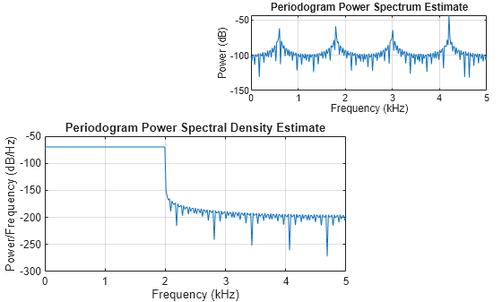

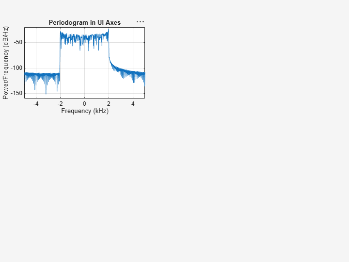
Plot Periodogram PSD Estimate in Target UI Axes

Create an axes in the northwestern corner of a new UI figure window.

uif = uifigure(Position=[100 100 720 540]);
ax3 = uiaxes(uif,Position=[5 305 300 200]);

Plot the periodogram PSD estimate of the signal x3 on the figure axes. Display the frequencies centered at 0 kHz.

periodogram(x3,g,nfft,Fs,"centered",Parent=ax3)
title(ax3,"Periodogram in UI Axes")

Plot Reassigned Periodogram PSD Estimate in Target Panel Container

Add a panel container in the southeastern corner of the UI figure window.

p = uipanel(uif,Position=[300 5 400 325], ...
    Title="Periodogram in Panel Container", ...
    BackgroundColor="white");

Plot the reassigned periodogram PSD estimate of the signal x4 on the panel container.

periodogram(x4,g,nfft,Fs,"reassigned",Parent=p)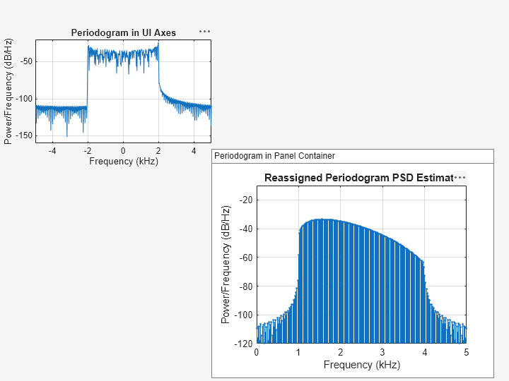

Input Arguments

x — Input signal

vector | matrix

Input signal, specified as a vector or as a matrix. If you specify x as a matrix, then periodogram treats its columns as independent channels.

Example: cos(pi/4*(0:159))+randn(1,160) is a single-channel row-vector signal.

Example: cos(pi./[4;2]*(0:159))'+randn(160,2) is a two-channel signal.

Data Types: single | double
Complex Number Support: Yes

win — Window

rectwin(length(x)) | kaiser(length(x),38) | vector | []

Window, specified as a row or column vector with the same length as the input signal. If you specify win as empty, then periodogram uses a rectangular window. If you specify the "reassigned" option and an empty win, then the function uses a Kaiser window with β = 38.

Note

The default rectangular window has a 13.3 dB sidelobe attenuation, which may mask spectral content below this value (relative to the peak spectral content). Choosing different windows enables you to make tradeoffs between resolution (for example, using a rectangular window) and sidelobe attenuation (for example, using a Hann window). See Window Designer for more details.

Data Types: single | double

freqSpec — Frequency specification

[] (default) | positive integer | vector

Frequency specification, specified as one of these values:

• Empty, [] — periodogram calculates the spectral estimates using a number of DFT points equal to the greater of 256 or the next power of two that is equal or larger than the window length.

• Positive integer — periodogram calculates the spectral estimates using the number of DFT points specified in this argument.

  • If freqSpec is greater than the segment length, then periodogram pads the segment data with zeros.

  • If freqSpec is less than the segment length, then periodogram partitions the segment modulo freqSpec and sums the resulting segment frames.

• Vector of at least two elements — periodogram calculates the spectral estimates at the frequencies specified in freqSpec.

  • If you specify the sample rate, Fs, periodogram assumes freqSpec as cyclical frequencies in the same units as of Fs.

  • If you do not specify Fs, periodogram assumes freqSpec as normalized frequencies in rad/sample.

Example: freqSpec = 512 specifies 512 DFT points.

Example: freqSpec = pi./[8 4 2] specifies a vector of three normalized frequencies.

Data Types: single | double

Fs — Sample rate

positive scalar

Sample rate, specified as a positive scalar. The sample rate is the number of samples per unit time. If the unit of time is seconds, then the sample rate is in Hz.

• If you specify Fs as empty [], then periodogram assumes that the input signal x has a sample rate of 1 Hz.

• If you do not specify Fs, then periodogram assumes that the input signal x has a sample rate of 2π rad/sample.

freqRange — Frequency range for PSD estimate or power spectrum

"onesided" | "twosided" | "centered"

Frequency range of the PSD estimate or power spectrum, specified as "onesided", "twosided", or "centered".

The periodogram function returns pxx with a number of rows and frequency interval that depends on the value specified in freqRange, whether the number of DFT points freqSpec is even or odd, and whether Fs is specified or not.

freqRange	freqSpec	Number of Rows in pxx	Frequency Interval for pxx
			Fs unspecified	Fs specified
"onesided" (default if x is real-valued)	Even	freqSpec/2 + 1	[0,π] rad/sample	[0,Fs/2] cycles/unit time
	Odd	(freqSpec + 1)/2	[0,π) rad/sample	[0,Fs/2) cycles/unit time
"twosided" (default if x is complex-valued)	Even or odd	freqSpec	[0,2π) rad/sample	[0,Fs) cycles/unit time
"centered"	Even	freqSpec	(–π,π] rad/sample	(–Fs/2,Fs/2] cycles/unit time
	Odd		(–π,π) rad/sample	(–Fs/2,Fs/2) cycles/unit time

Note

• This argument is not supported if you specify freqSpec as a vector of cyclical or normalized frequencies.

• If you specify the "onesided" value, periodogram multiplies the power by 2 at all frequencies except 0 and the Nyquist frequency to conserve the total power.

• The "onesided" value is not supported if x is complex-valued.

Data Types: char | string

spectrumType — Power spectrum scaling

"psd" (default) | "power"

Power spectrum scaling, specified as one of these values:

• "psd" — periodogram returns the power spectral density.

• "power" — periodogram scales each estimate of the PSD by the equivalent noise bandwidth of the window and returns an estimate of the power at each frequency. If you also specify "reassigned", periodogram integrates the PSD over the width of each frequency bin before reassigning.

This table shows the scaling relation between the PSD estimate and power spectrum estimate, either of both returned in pxx, given an input signal x, window vector win, frequency specification freqSpec, and sample rate Fs.

Sample Rate	Scaling relation
Fs specified	[~,~,~,psd] = periodogram(x,win,freqSpec,Fs,"psd"); [~,~,~,pow] = periodogram(x,win,freqSpec,Fs,"power"); Then, pow is equivalent to psd*enbw(win,Fs).
Fs unspecified	[~,~,~,psd] = periodogram(x,win,freqSpec,"psd"); [~,~,~,pow] = periodogram(x,win,freqSpec,"power"); Then, pow is equivalent to psd*enbw(win,2*pi).

Data Types: char | string

p — Confidence interval for PSD estimate

0.95 (default) | scalar in the range (0,1)

Coverage probability for the PSD estimate, specified as a scalar in the range (0,1).

If you specify ConfidenceLevel=p and pxxc, the function outputs pxxc with the lower and upper bounds of the p × 100% interval estimate for the true PSD.

h — Target parent container

[] (default) | Axes object | UIAxes object | Panel object

Since R2026a

Target parent container, specified as an Axes object, a UIAxes object, or a Panel object.

If you specify Parent=h, the periodogram function plots the periodogram PSD estimate or power spectrum on the specified target parent container, whether you call the function with or without output arguments.

For more information about target containers and the parent-child relationship in MATLAB^® graphics, see Graphics Object Hierarchy. For more information about using Parent in UIAxes and Panel objects to design apps, see Plot Spectral Representations of Signal in App Designer.

Example: h = axes(figure,Position=[0.1 0.1 0.6 0.5]) defines an axes parent container. When you specify periodogram(x,[],[],[],Parent=h), the function plots the periodogram PSD of the input signal x in the parent container h.

Output Arguments

pxx — PSD estimate or power spectrum

vector | matrix

PSD estimate or power spectrum, returned as a real-valued, nonnegative column vector or matrix.

• Each column of pxx is the PSD estimate or the or power spectrum of the corresponding column of x and depending on how you specify spectrumType.

• The units of the PSD estimate are in squared-magnitude units of the input signal per unit frequency. For example, if the input data x is in volts, you specify the sample rate Fs in hertz, and you assume a resistance of 1 Ω, then the PSD estimate is in watts per hertz.

• The units of the power spectrum are in squared-magnitude units of the input signal. For example, if the input data x is in volts and you assume a resistance of 1 Ω, then the PSD estimate is in watts.

f — Frequencies associated with PSD estimate

vector

Frequencies associated with the PSD estimate, returned as a real-valued column vector.

• If you specify Fs, then f contains cyclical frequencies in Hz.

• If you do not specify Fs, then f contains normalized frequencies in rad/sample.

pxxc — Confidence bounds

matrix

Confidence bounds, returned as a real-valued matrix.

• pxxc has the same number of rows as in pxx.

• pxxc has twice as many columns as pxx.

  • Odd-numbered columns contain the lower bounds of the confidence intervals.

  • Even-numbered columns contain the upper bounds of the confidence intervals.

  Thus, pxxc(m,2*n-1) is the lower confidence bound and pxxc(m,2*n) is the upper confidence bound corresponding to the estimate pxx(m,n).

• The coverage probability of the confidence intervals is determined by the value of the p input.

Data Types: single | double

rpxx — Reassigned PSD estimate

vector | matrix

Reassigned PSD estimate, returned as a real-valued, nonnegative column vector or matrix. Each column of rpxx is the reassigned PSD estimate of the corresponding column of x.

fc — Center-of-energy frequencies

vector | matrix

Center-of-energy frequencies, returned as a vector or matrix.

More About

Periodogram

The periodogram is a nonparametric estimate of the power spectral density (PSD) of a wide-sense stationary random process. The periodogram is the Fourier transform of the biased estimate of the autocorrelation sequence. For a signal x_n sampled at Fs samples per unit time, the periodogram is defined as

$$\widehat{P}(f)=\frac{\Delta t}{N}{\left|{\displaystyle \sum _{n=0}^{N-1}{x}_n}{e}^{-j2\pi f\Delta tn}\right|}^2,-1/2\Delta t<f\le 1/2\Delta t,$$

where Δt is the sampling interval. For a one-sided periodogram, the values at all frequencies except 0 and the Nyquist, 1/2Δt, are multiplied by 2 so that the total power is conserved.

If the frequencies are in radians per sample, the periodogram is defined as

$$\widehat{P}(\omega )=\frac{1}{2\pi N}{\left|{\displaystyle \sum _{n=0}^{N-1}{x}_n}{e}^{-j\omega n}\right|}^2,-\pi <\omega \le \pi .$$

The frequency range in the preceding equations has variations depending on the value of the freqRange argument. See the description of freqRange in Input Arguments.

The integral of the true PSD, P(f), over one period, 1/Δt for cyclical frequency and 2π for normalized frequency, is equal to the variance of the wide-sense stationary random process:

$${\sigma }^2={\displaystyle {\int }_{-1/2\Delta t}^{1/2\Delta t}P}(f)df.$$

For normalized frequencies, replace the limits of integration appropriately.

Modified Periodogram

The modified periodogram multiplies the input time series by a window function. A suitable window function is nonnegative and decays to zero at the beginning and end points. Multiplying the time series by the window function tapers the data gradually on and off and helps to alleviate the leakage in the periodogram. See Bias and Variability in the Periodogram for an example.

If h_n is a window function, the modified periodogram is defined by

$$\widehat{P}(f)=\frac{\Delta t}{N}{\left|{\displaystyle \sum _{n=0}^{N-1}{h}_n}{x}_n{e}^{-j2\pi f\Delta tn}\right|}^2,-1/2\Delta t<f\le 1/2\Delta t,$$

where Δt is the sampling interval.

If the frequencies are in radians per sample, the modified periodogram is defined as

$$\widehat{P}(\omega )=\frac{1}{2\pi N}{\left|{\displaystyle \sum _{n=0}^{N-1}{h}_n}{x}_n{e}^{-j\omega n}\right|}^2,-\pi <\omega \le \pi .$$

The frequency range in the preceding equations has variations depending on the value of the freqRange argument. See the description of freqRange in Input Arguments.

Reassigned Periodogram

The reassignment technique sharpens the localization of spectral estimates and produces periodograms that are easier to read and interpret. This technique reassigns each PSD estimate to the center of energy of its bin, away from the bin’s geometric center. It provides exact localization for chirps and impulses.

References

[1] Auger, François, and Patrick Flandrin. "Improving the Readability of Time-Frequency and Time-Scale Representations by the Reassignment Method." IEEE^® Transactions on Signal Processing. Vol. 43, May 1995, pp. 1068–1089.

[2] Fulop, Sean A., and Kelly Fitz. "Algorithms for computing the time-corrected instantaneous frequency (reassigned) spectrogram, with applications." Journal of the Acoustical Society of America. Vol. 119, January 2006, pp. 360–371.

Extended Capabilities

C/C++ Code Generation
Generate C and C++ code using MATLAB® Coder™.

GPU Code Generation
Generate CUDA® code for NVIDIA® GPUs using GPU Coder™.

GPU Arrays

Accelerate code by running on a graphics processing unit (GPU) using Parallel Computing Toolbox™.

This function fully supports GPU arrays. For more information, see Run MATLAB Functions on a GPU (Parallel Computing Toolbox).

Version History

Introduced before R2006a

R2026a: Visualize function outputs in specified parent targets

The periodogram function supports plotting output in a parent axes or panel container specified using the Parent input argument.

R2024a: Code generation support for single-precision variable-size window inputs

The periodogram function supports single-precision variable-size window inputs for code generation.

R2024a: periodogram supports GPU code generation

The periodogram function supports code generation for graphical processing units (GPUs). You must have MATLAB Coder™ and GPU Coder™ to generate CUDA^® code.

R2023b: Use single-precision data

The periodogram function supports single-precision inputs.

R2023a: Visualize function outputs using Create Plot Live Editor task

You can now use the Create Plot Live Editor task to visualize the output of periodogram interactively. You can select different chart types and set optional parameters. The task also automatically generates code that becomes part of your live script.