Multi-Stage Rolling Mill Simulation and Control

R2026b

Since R2026b

This example shows how to simulate a multi-stage foil rolling mill using Simulink® and Simscape™. The model combines a physically grounded rolling process with closed-loop thickness and velocity control to enable analysis of both deformation physics and control behavior. The model represents a two-stage rolling mill that progressively reduces the thickness of the foil from 40 mm to 10 mm, coordinating DC motor drives, hydraulic actuators, and a looper mechanism to maintain precise gauge control while conserving mass flow.

In this example, you:

• Open a Simscape Multibody™ rolling mill model with custom foil domain components.

• Initialize physical plant parameters, controller gains, and hydraulic actuator settings.

• Simulate the closed-loop system for 10 seconds of rolling operation.

• Verify that thickness controllers converge to their gauge targets at each stand.

• Confirm mass flow conservation across all roller stages.

• Examine motor torques, rolling forces, and looper behavior during transients.

This example runs the model in Simscape Multibody™ Explorer so you can observe the foil thickness change over time.

Open and Explore Model

To inspect the model before simulation, load the project and open the multiStageRollingMill model. The model integrates mechanical roller dynamics, elastic foil spans, DC motor armature circuits, and hydraulic automatic gauge control (AGC) in a single feedback configuration.

matlab.project.loadProject(fullfile(pwd, 'multiStageRollingMill'));
mdl = 'multiStageRollingMill';
open_system(mdl);
simulinkScreenshot(mdl);

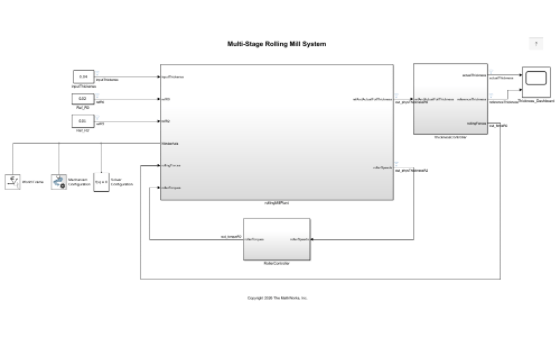
To look at the physical plant model that captures the mechanical deformation and rolling dynamics, open the rollingMillPlant subsystem.

blk = mdl + "/rollingMillPlant";
simulinkScreenshot(blk);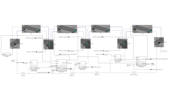

System Architecture

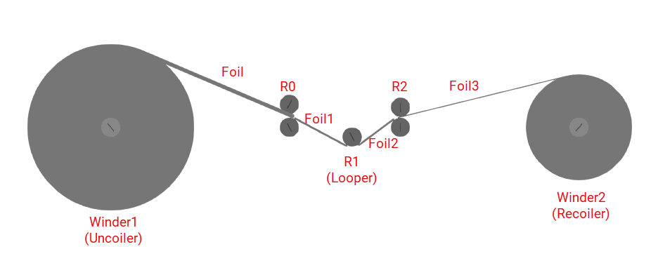
The rolling mill consists of five mechanical elements arranged in a line. Two winders (uncoiler and recoiler) feed and collect the foil, while three rollers progressively reduce foil thickness. Winder1 uncoils the foil. Roller0 (R0), which consists of a top and bottom roller, reduces the foil from 40 mm (Foil) to 20 mm (Foil1). Roller1 (R1) acts as a passive looper that resists the motion to maintain inter-stand tension with constant foil thickness (Foil1 to Foil2). Roller2 (R2) also consists of a top and bottom roller and performs the final reduction from 20 mm (Foil2) to 10 mm (Foil3). Winder2 recoils the finished foil.

Main Subsystems	Subsystem Name	Description
Mechanical plant	rollingMillPlant	Models rollers, foil, and winders using Simscape Multibody™ and handles physical deformation and motion
Roller velocity control	RollerController	A PI controller commands a DC motor to maintain constant roller angular velocity.
Thickness control	ThicknessController	A PID controller commands a hydraulic press to achieve the target foil thickness via the prismatic joint gap. Thickness feedback comes directly from the NipContact estimator of the top roller.
Looper control	LooperPI	Maintains proper tension between stages and adjusts downstream speed dynamically
Nip contact model	NipContact	Uses Bland-Ford theory to compute rolling force and deformation

Initialize Parameters and Simulate

To configure the simulation with physically realistic values, run the initialization script. This script defines the roller geometry, foil material properties, DC motor electrical parameters, hydraulic actuator dynamics, and controller gains. The roller radius and foil thickness targets determine the required speed ratios between stands. The yield stress governs the Bland-Ford rolling force magnitude.

rollingMillRollerInitialization;

Roller control parameters set.

out = sim('multiStageRollingMill');

Analyze Results

The simulation shows that thickness converges to targets, mass flow is conserved across stages, and roller speeds follow expected ratios. The model generates realistic rolling forces and motor torques, and the looper stabilizes the tension between stages.

Verify Foil Thickness Convergence

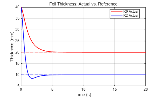
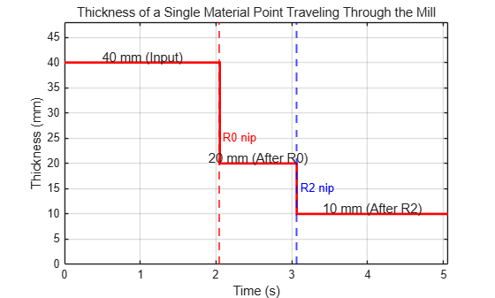
Compare the actual foil thickness against the reference target across time. To verify that the hydraulic AGC achieves the target gauge at each stand, plot the physical thickness measured at the nip exit of R0 and R2. Both thickness controllers converge to their setpoints in approximately 4 seconds. The R0 stand reduces the foil from 40 mm to the 20 mm target. R2 further reduces the foil to the final 10 mm target.

plotThicknessTracking;

Verify Mass Flow Conservation

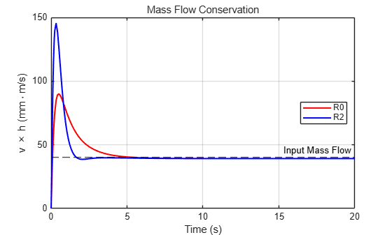
To confirm that the control system maintains consistent mass flow, compute the product of surface speed, $$v$$, and thickness, $$h$$, at each stand. For incompressible material, $$v\times h$$ (surface speed times thickness) must remain constant across all stands. The reference velocity at each stand is derived from this constraint, coupling thickness reduction to roller speed.

Both stands in this example converge to the same mass flow invariant of 0.04 m^2/s. The transient overshoot reflects the velocity PI controllers driving open-loop dynamics to equilibrium. The custom ElasticFoil Simscape component uses a speed_ratio parameter that encodes the expected velocity ratio so that the foil generates tension only from deviations from the mass flow conserving speed, not from the nominal speed.

plotMassFlowConservation;

Hydraulic Correction Forces

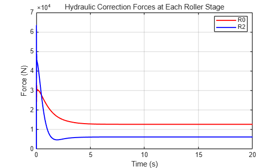
The thickness control loop ThicknessController outputs the hydraulic correction forces. These correction forces are applied to the prismatic joint of each stand to adjust the rollers to create the precise gap required for foil thickness adjustments.

plotHydraulicForces;

Verify Roller Speed Ratios and Forces

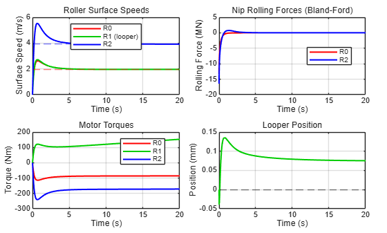
Examine the roller surface speeds, nip forces, motor torques, and looper behavior during transient and steady-state operation.

plotRollingMillResults;

--- Rolling Mill Results Summary ---
Speed:       R0 = 1.96 m/s,  R1 = 1.96 m/s,  R2 = 3.92 m/s
Speed ratio: R2/R0 = 2.00 (target 2.0)
Forces:      R0 = 13416 kN,  R2 = 16432 kN
-----------------------------------

These plots show:

• Roller surface speeds follow the expected mass-flow relationship. In steady state, R2 operates at approximately twice the surface speed of R0, consistent with the thickness reduction across the two rolling stages.

• Nip forces are nonzero during the transient period when the rollers actively reduce foil thickness. As the system approaches steady state and the incoming foil reaches the target gauge, the required deformation decreases and the separating force converges to zero.

• Motor torques reflect both direction and load distribution across the rollers. R1 rotates in the opposite direction to R0 and R2, and torque magnitude increases slightly in downstream rollers due to higher surface speeds.

• Looper behavior regulates inter-stand tension rather than thickness. Looper torque reflects the tension difference between adjacent spans along with inertia and damping effects. Looper position provides a useful indicator of system performance: a well-tuned system shows a brief transient excursion followed by a smooth return to nominal, indicating stable tension regulation.

Physical Components

The model uses a custom Simscape library (+Rollers) that defines a foil domain with across variables including radius, angle, angular velocity, and tangential contact point quantities, and a through variable, torque. This domain enables modular connections between roller and foil components. For definitions of the variables used in equations in this model, see Equation Variables.

Roller Stands (Roller0, Roller1, Roller2)

The roller assemblies are modeled with Simscape Multibody. Bottom rollers are driven by DC motor torque through revolute joints. Each stand has a prismatic joint that converts the hydraulic correction force into vertical displacement of the bottom roller, adjusting the roller gap for thickness control.

Top Rollers (TopRoller_R0, TopRoller_R2)

Each top roller sits on a prismatic joint that allows vertical positioning to control the roller gap. Nip contact force is computed using the Bland-Ford rolling force model: $$F_{sep}=Q_p\cdot {\sigma }_y\cdot w\cdot L_d$$, where $$L_d=\sqrt{R_{roll}\cdot \Delta h}$$.

Winders (Winder1, Winder2)

Winder1 uncoils the feed stock and Winder2 recoils the finished foil. Both maintain strip tension using the custom Angle2Radius Simscape component.

Elastic Foil Sections (Foil, Foil1, Foil2, Foil3)

Each foil span transmits position and torque between adjacent components. Span tension combines elastic stretch and viscous damping: $$F=\frac{\Delta L\cdot E_t+\Delta \underset{}{\overset{\dot{}}{L}}\cdot D}{L_0}\cdot t_h\cdot w+F_0$$.

Control Architecture

The system uses two separate controller subsystems operating in parallel, with the additional winder controller WinderCtrl that maintains strip tension at the entry and exit of the mill.

Velocity Control (RollerController)

Each stand has an independent speed control loop (Vel Ctrl R0, Vel Ctrl R2). Each stand's speed reference is derived from mass flow conservation: $${\omega }_{ref}=V_{ref}\cdot (T_{input}/T_{target})/R_{roll}$$. A rate limiter (±300 rad/s²) smooths startup. The controller outputs armature voltage to the DC motor. R1 (the looper) does not use a fixed reference; its speed is adjusted dynamically by the looper controller.

Looper Controller (LooperPI)

A PID compensator regulates the looper position (strip tension between stands). The compensator measures the looper deflection angle and adjusts the speed reference of downstream roller R2 to maintain proper inter-stand tension. The compensator also includes anti-windup and saturation logic.

Thickness Control (ThicknessController)

Each rolling stand has an Automatic Gauge Control (AGC) layer. The AGC layer receives thickness feedback from the top roller's NipContact estimator, applies a PID controller, and commands the hydraulic actuator to position the bottom roller via the prismatic joint at each stand.

Equation Variables

These variables are used in the equations referenced throughout this example.

Variable	Description
$$F_{sep}$$	Separating force between rollers
$$Q_p$$	Geometry factor accounting for friction and contact pressure distribution
$${\sigma }_y$$	Material yield stress of foil
$$w$$	Foil width
$$L_d$$	Projected contact arc length
$$R_{roll}$$	Roller radius
$$\Delta h$$	Draft (reduction in thickness)
$$\Delta L$$	Total stretch of foil (rotational + positional - tangential contact change)
$$E_t$$	Tension modulus of foil
$$D$$	Damping modulus of foil
$$L_0$$	Initial span length of foil
$$F$$	Foil tension force
$$F_0$$	Initial pretension force in foil
$$\Delta \underset{}{\overset{\dot{}}{L}}$$	Rate of change of foil stretch (velocity difference)
$$t_h$$	Foil thickness
$${\omega }_{ref}$$	Reference angular velocity for the roller
$$V_{ref}$$	Reference foil surface speed at the input
$$T_{input}$$	Foil thickness at the input
$$T_{target}$$	Target exit thickness at a given stand

Summary

The multi-stage rolling mill system modeled in this example shows:

• The Custom Simscape domain (+Rollers/foil.ssc) enables modular roller-foil connections with physically meaningful across and through variables.

• Top and bottom roller pairs with Bland-Ford nip contact model compute realistic rolling forces at each stand.

• Parallel control architecture with a velocity PI loop (RollerController) and a thickness PID loop (ThicknessController) achieves the target foil thickness to tight tolerances.

• Hydraulic gap control with prismatic joints converts correction forces into precise roller gap adjustments at each stand.

• Mass flow conservation through the speed_ratio parameter in ElasticFoil.ssc enables correct inter-stand speed ratios (R2 runs at 2x the surface speed of R0).

• The model reduces foil from 40 mm to 10 mm across two rolling stands with a looper (40 → 20 → 10 mm).