Résultats pour

 $ is the unknown displacement of the oscillator occupying the n-th position of the lattice, and
 and
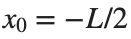
and 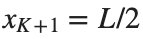 , that is,
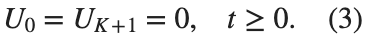
 for the one-dimensional discrete Laplacian
 . We consider spatially extended initial conditions of the form:
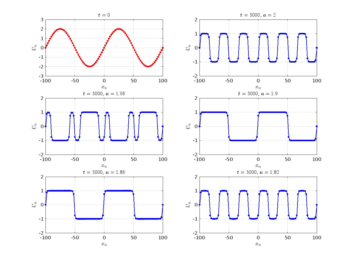
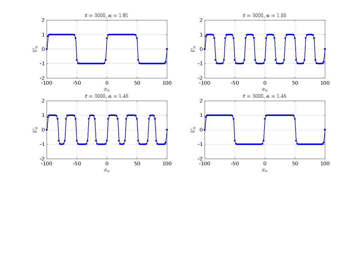
 where the dynamics appear in the first image of the third row, we observe convergence to a non-linear equilibrium point of branch
  respectively, converges to a non-linear equilibrium point of branch
  and energy
 - Tips & tricks: Discuss strategies for solving Cody problems that you've found effective.
- Ideas or suggestions for improvement: Have thoughts on how to make Cody better? We'd love to hear them.
- Issues: Encountering difficulties or bugs with Cody? Let us know so we can address them.
- Requests for guidance: Stuck on a Cody problem? Ask for advice or hints, but make sure to show your efforts in attempting to solve the problem first.
- General discussions: Anything else related to Cody that doesn't fit into the above categories.
- Comments on specific Cody problems: Examples include unclear problem descriptions or incorrect testing suites.
- Comments on specific Cody solutions: For example, you find a solution creative or helpful.
- Exclusive Hands-On Experience: Be among the first to explore new MATLAB features and capabilities.
- Voice Your Expertise: Share your insights and suggestions directly with MathWorks developers.
- Learn, Discover, and Grow: Expand your MATLAB knowledge and skills through firsthand experience with unreleased features.
- Network Over Dinner: Enjoy a complimentary dinner with fellow MATLAB enthusiasts and the MathWorks team. It's a perfect opportunity to connect, share experiences, and network after work.
- Earn Rewards: Participants will not only contribute to the advancement of MATLAB but will also be compensated for their time. Plus, enjoy special MathWorks swag as a token of our appreciation!


- Create a criptocurrency strategy algorythm (for buying and selling some crypto like BTC, ETH etc).
- Backtesting the strategy with historical data (I've a bunch of json files with different timeframes, downloaded with freqtrade from binance).
- Optimize the strategy given some parameters (they can be numeric, like ROI, some kind of enumeration, like "selltype" and so on).
- Convert the strategy algorithm in python, so I can use it with Freqtrade without worrying of manually copying formulas and parameters that's error prone.
- I'd like to write both classic algorithm and some deep neural one, that try to find best strategy with little neural network (they should run on my pc with 32gb of ram and a 3080RTX if it can be gpu accelerated).

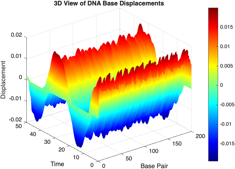
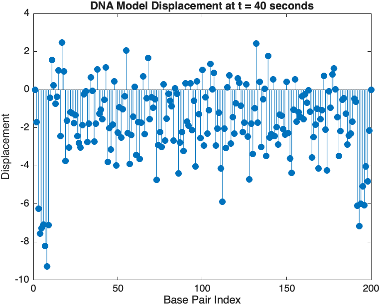
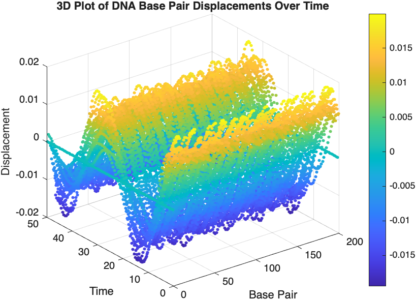
- Position: Random initial perturbations between 0.01 and 0.02 to simulate the thermal fluctuations at the start.
- Velocity: All bases start from rest, assuming no initial movement except for the thermal perturbations.
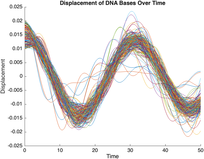
- Wave Propagation: The initial perturbations lead to wave-like dynamics along the segment, with visible propagation and reflection at the boundaries.
- Damping Effects: The inclusion of damping leads to a gradual reduction in the amplitude of the oscillations, indicating energy dissipation over time.
- Nonlinear Behavior: The nonlinear term influences the response, potentially stabilizing the system against large displacements or leading to complex dynamic patterns.
Hello MathWorks Community,
I am excited to announce that I am currently working on a book project centered around Matrix Algebra, specifically designed for MATLAB users. This book aims to cater to undergraduate students in engineering, where Matrix Algebra serves as a foundational element.
Matrix Algebra is not only pivotal in understanding complex engineering concepts but also in applying these principles effectively in various technological solutions. MATLAB, renowned for its powerful computational capabilities, is an excellent tool to explore and implement these concepts, making it a perfect companion for this book.
As I embark on this journey to create a resource that bridges theoretical matrix algebra with practical MATLAB applications, I am looking for one or two knowledgeable individuals who have a firm grasp of both subjects. If you have experience in teaching or applying matrix algebra in engineering contexts and are familiar with MATLAB, your contribution could be invaluable.
Collaborators will help in shaping the content to ensure it is educational, engaging, and technically robust, making complex concepts accessible and applicable for students.
If you are interested in contributing to this project or know someone who might be, please reach out to discuss how we can work together to make this book a valuable resource for engineering students.
Thank you and looking forward to your participation!