Résultats pour
While searching the internet for some books on ordinary differential equations, I came across a link that I believe is very useful for all math students and not only. If you are interested in ODEs, it's worth taking the time to study it.
A First Look at Ordinary Differential Equations by Timothy S. Judson is an excellent resource for anyone looking to understand ODEs better. Here's a brief overview of the main topics covered:
- Introduction to ODEs: Basic concepts, definitions, and initial differential equations.
- Methods of Solution:
- Separable equations
- First-order linear equations
- Exact equations
- Transcendental functions
- Applications of ODEs: Practical examples and applications in various scientific fields.
- Systems of ODEs: Analysis and solutions of systems of differential equations.
- Series and Numerical Methods: Use of series and numerical methods for solving ODEs.
This book provides a clear and comprehensive introduction to ODEs, making it suitable for students and new researchers in mathematics. If you're interested, you can explore the book in more detail here: A First Look at Ordinary Differential Equations.
The study of the dynamics of the discrete Klein - Gordon equation (DKG) with friction is given by the equation :

above equation, W describes the potential function :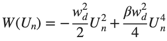
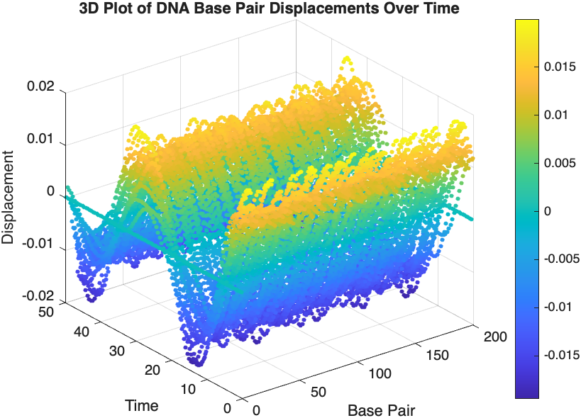
The objective of this simulation is to model the dynamics of a segment of DNA under thermal fluctuations with fixed boundaries using a modified discrete Klein-Gordon equation. The model incorporates elasticity, nonlinearity, and damping to provide insights into the mechanical behavior of DNA under various conditions.
% Parameters
numBases = 200; % Number of base pairs, representing a segment of DNA
kappa = 0.1; % Elasticity constant
omegaD = 0.2; % Frequency term
beta = 0.05; % Nonlinearity coefficient
delta = 0.01; % Damping coefficient
- Position: Random initial perturbations between 0.01 and 0.02 to simulate the thermal fluctuations at the start.
- Velocity: All bases start from rest, assuming no initial movement except for the thermal perturbations.
% Random initial perturbations to simulate thermal fluctuations
initialPositions = 0.01 + (0.02-0.01).*rand(numBases,1);
initialVelocities = zeros(numBases,1); % Assuming initial rest state
The simulation uses fixed ends to model the DNA segment being anchored at both ends, which is typical in experimental setups for studying DNA mechanics. The equations of motion for each base are derived from a modified discrete Klein-Gordon equation with the inclusion of damping:
% Define the differential equations
dt = 0.05; % Time step
tmax = 50; % Maximum time
tspan = 0:dt:tmax; % Time vector
x = zeros(numBases, length(tspan)); % Displacement matrix
x(:,1) = initialPositions; % Initial positions
% Velocity-Verlet algorithm for numerical integration
for i = 2:length(tspan)
% Compute acceleration for internal bases
acceleration = zeros(numBases,1);
for n = 2:numBases-1
acceleration(n) = kappa * (x(n+1, i-1) - 2 * x(n, i-1) + x(n-1, i-1)) ...
- delta * initialVelocities(n) - omegaD^2 * (x(n, i-1) - beta * x(n, i-1)^3);
end
% positions for internal bases
x(2:numBases-1, i) = x(2:numBases-1, i-1) + dt * initialVelocities(2:numBases-1) ...
+ 0.5 * dt^2 * acceleration(2:numBases-1);
% velocities using new accelerations
newAcceleration = zeros(numBases,1);
for n = 2:numBases-1
newAcceleration(n) = kappa * (x(n+1, i) - 2 * x(n, i) + x(n-1, i)) ...
- delta * initialVelocities(n) - omegaD^2 * (x(n, i) - beta * x(n, i)^3);
end
initialVelocities(2:numBases-1) = initialVelocities(2:numBases-1) + 0.5 * dt * (acceleration(2:numBases-1) + newAcceleration(2:numBases-1));
end
% Visualization of displacement over time for each base pair
figure;
hold on;
for n = 2:numBases-1
plot(tspan, x(n, :));
end
xlabel('Time');
ylabel('Displacement');
legend(arrayfun(@(n) ['Base ' num2str(n)], 2:numBases-1, 'UniformOutput', false));
title('Displacement of DNA Bases Over Time');
hold off;
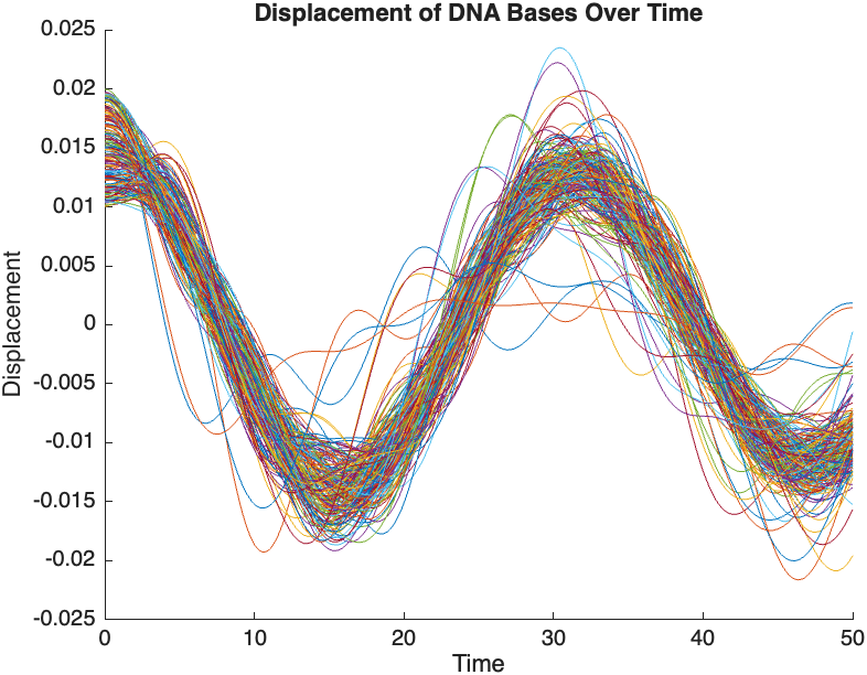
The results are visualized using a plot that shows the displacements of each base over time . Key observations from the simulation include :
- Wave Propagation: The initial perturbations lead to wave-like dynamics along the segment, with visible propagation and reflection at the boundaries.
- Damping Effects: The inclusion of damping leads to a gradual reduction in the amplitude of the oscillations, indicating energy dissipation over time.
- Nonlinear Behavior: The nonlinear term influences the response, potentially stabilizing the system against large displacements or leading to complex dynamic patterns.
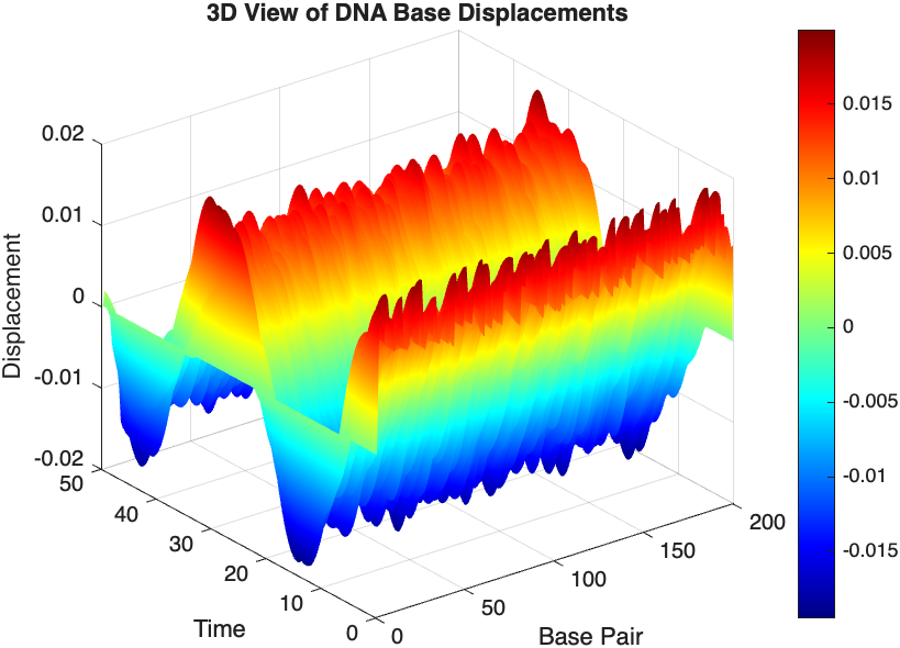
% 3D plot for displacement
figure;
[X, T] = meshgrid(1:numBases, tspan);
surf(X', T', x);
xlabel('Base Pair');
ylabel('Time');
zlabel('Displacement');
title('3D View of DNA Base Displacements');
colormap('jet');
shading interp;
colorbar; % Adds a color bar to indicate displacement magnitude
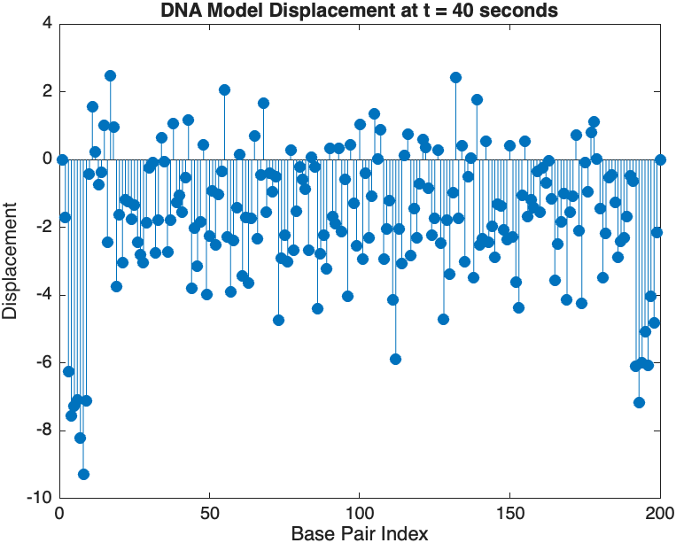
% Snapshot visualization at a specific time
snapshotTime = 40; % Desired time for the snapshot
[~, snapshotIndex] = min(abs(tspan - snapshotTime)); % Find closest index
snapshotSolution = x(:, snapshotIndex); % Extract displacement at the snapshot time
% Plotting the snapshot
figure;
stem(1:numBases, snapshotSolution, 'filled'); % Discrete plot using stem
title(sprintf('DNA Model Displacement at t = %d seconds', snapshotTime));
xlabel('Base Pair Index');
ylabel('Displacement');
% Time vector for detailed sampling
tDetailed = 0:0.5:50; % Detailed time steps
% Initialize an empty array to hold the data
data = [];
% Generate the data for 3D plotting
for i = 1:numBases
% Interpolate to get detailed solution data for each base pair
detailedSolution = interp1(tspan, x(i, :), tDetailed);
% Concatenate the current base pair's data to the main data array
data = [data; repmat(i, length(tDetailed), 1), tDetailed', detailedSolution'];
end
% 3D Plot
figure;
scatter3(data(:,1), data(:,2), data(:,3), 10, data(:,3), 'filled');
xlabel('Base Pair');
ylabel('Time');
zlabel('Displacement');
title('3D Plot of DNA Base Pair Displacements Over Time');
colorbar; % Adds a color bar to indicate displacement magnitude
I'm excited to share some valuable resources that I've found to be incredibly helpful for anyone looking to enhance their MATLAB skills. Whether you're just starting out, studying as a student, or are a seasoned professional, these guides and books offer a wealth of information to aid in your learning journey.
These materials are freely available and can be a great addition to your learning resources. They cover a wide range of topics and are designed to help users at all levels to improve their proficiency in MATLAB.
Happy learning and I hope you find these resources as useful as I have!
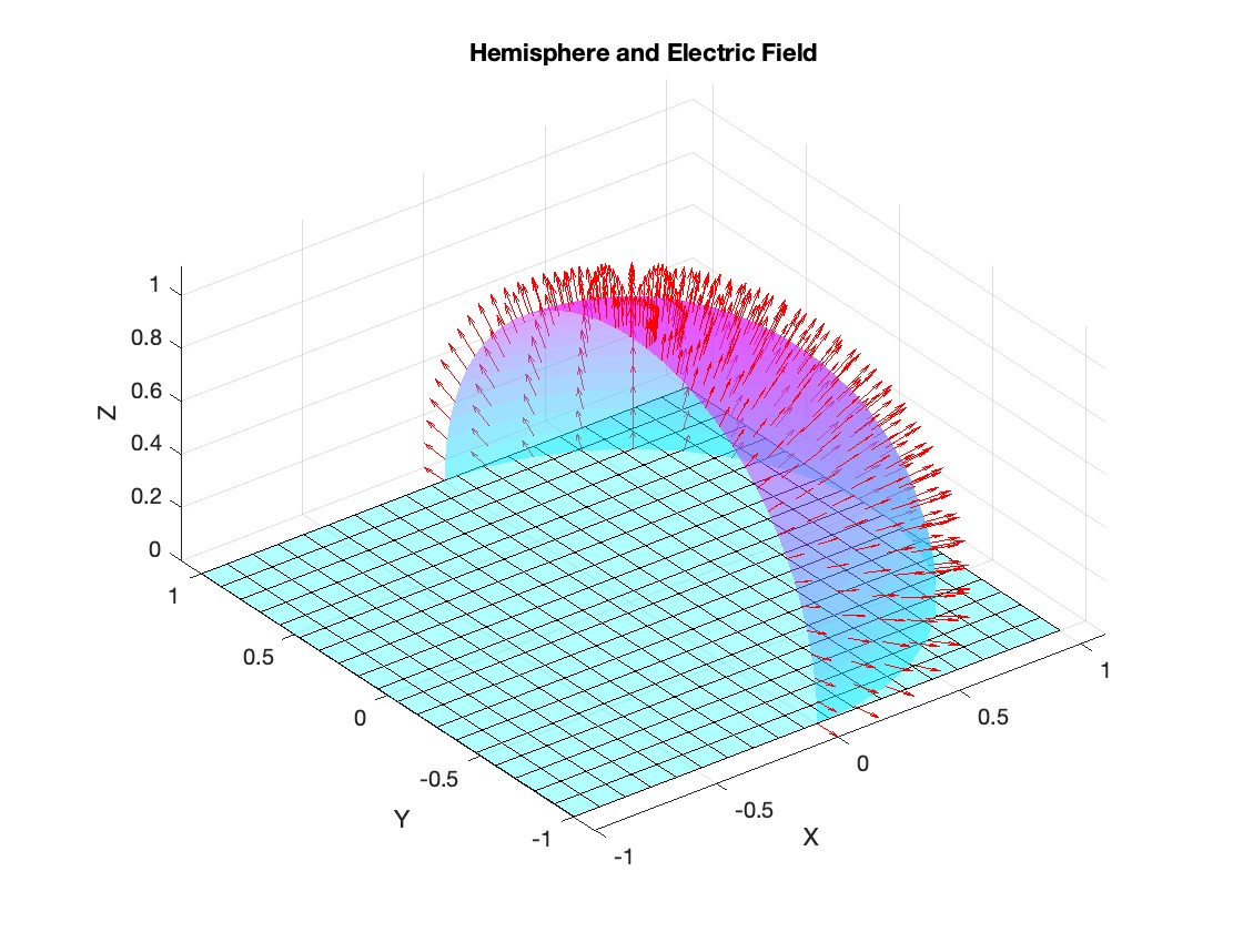
Let S be the closed surface composed of the hemisphere  and the base
  Let
Let  be the electric field defined by
  . Find the electric flux through S. (Hint: Divide S into two parts and calculate
  ).
).
% Define the limits of integration for the hemisphere S1
theta_lim = [-pi/2, pi/2];
phi_lim = [0, pi/2];
% Perform the double integration over the spherical surface of the hemisphere S1
% Define the electric flux function for the hemisphere S1
flux_function_S1 = @(theta, phi) 2 * sin(phi);
electric_flux_S1 = integral2(flux_function_S1, theta_lim(1), theta_lim(2), phi_lim(1), phi_lim(2));
% For the base of the hemisphere S2, the electric flux is 0 since the electric
% field has no z-component at the base
electric_flux_S2 = 0;
% Calculate the total electric flux through the closed surface S
total_electric_flux = electric_flux_S1 + electric_flux_S2;
% Display the flux calculations
disp(['Electric flux through the hemisphere S1: ', num2str(electric_flux_S1)]);
disp(['Electric flux through the base of the hemisphere S2: ', num2str(electric_flux_S2)]);
disp(['Total electric flux through the closed surface S: ', num2str(total_electric_flux)]);
% Parameters for the plot
radius = 1; % Radius of the hemisphere
% Create a meshgrid for theta and phi for the plot
[theta, phi] = meshgrid(linspace(theta_lim(1), theta_lim(2), 20), linspace(phi_lim(1), phi_lim(2), 20));
% Calculate Cartesian coordinates for the points on the hemisphere
x = radius * sin(phi) .* cos(theta);
y = radius * sin(phi) .* sin(theta);
z = radius * cos(phi);
% Define the electric field components
Ex = 2 * x;
Ey = 2 * y;
Ez = 2 * z;
% Plot the hemisphere
figure;
surf(x, y, z, 'FaceAlpha', 0.5, 'EdgeColor', 'none');
hold on;
% Plot the electric field vectors
quiver3(x, y, z, Ex, Ey, Ez, 'r');
% Plot the base of the hemisphere
[x_base, y_base] = meshgrid(linspace(-radius, radius, 20), linspace(-radius, radius, 20));
z_base = zeros(size(x_base));
surf(x_base, y_base, z_base, 'FaceColor', 'cyan', 'FaceAlpha', 0.3);
% Additional plot settings
colormap('cool');
axis equal;
grid on;
xlabel('X');
ylabel('Y');
zlabel('Z');
title('Hemisphere and Electric Field');
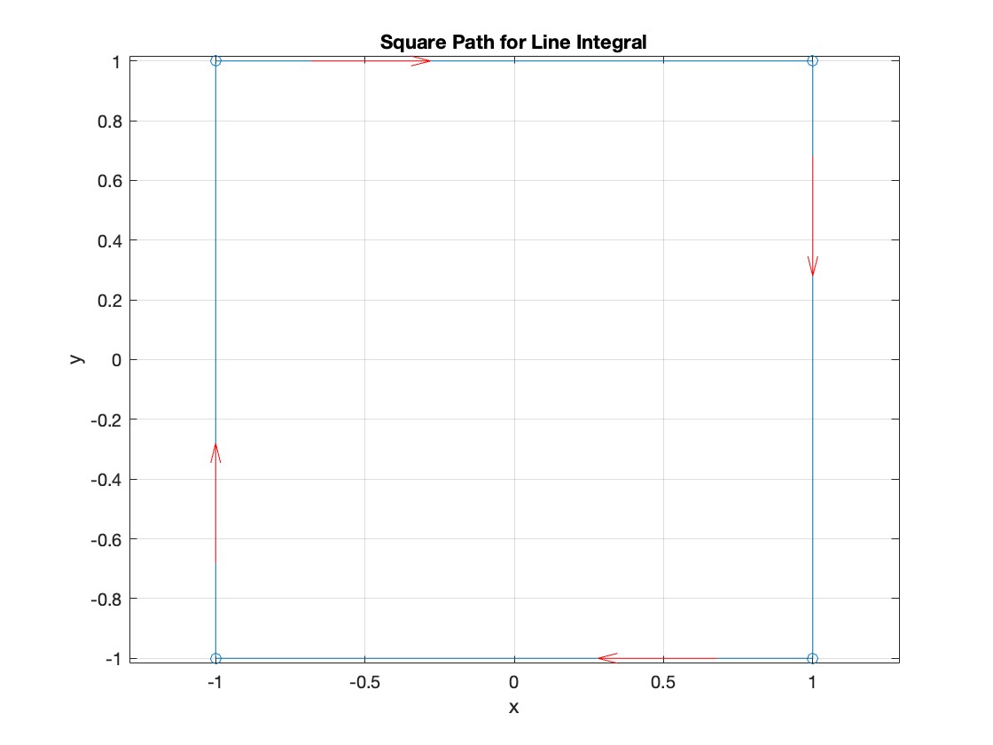
The line integral  , where C is the boundary of the square
  oriented counterclockwise, can be evaluated in two ways:
, where C is the boundary of the square Using the definition of the line integral:
% Initialize the integral sum
integral_sum = 0;
% Segment C1: x = -1, y goes from -1 to 1
y = linspace(-1, 1);
x = -1 * ones(size(y));
dy = diff(y);
integral_sum = integral_sum + sum(-x(1:end-1) .* dy);
% Segment C2: y = 1, x goes from -1 to 1
x = linspace(-1, 1);
y = ones(size(x));
dx = diff(x);
integral_sum = integral_sum + sum(y(1:end-1).^2 .* dx);
% Segment C3: x = 1, y goes from 1 to -1
y = linspace(1, -1);
x = ones(size(y));
dy = diff(y);
integral_sum = integral_sum + sum(-x(1:end-1) .* dy);
% Segment C4: y = -1, x goes from 1 to -1
x = linspace(1, -1);
y = -1 * ones(size(x));
dx = diff(x);
integral_sum = integral_sum + sum(y(1:end-1).^2 .* dx);
disp(['Direct Method Integral: ', num2str(integral_sum)]);
Plotting the square path
% Define the square's vertices
vertices = [-1 -1; -1 1; 1 1; 1 -1; -1 -1];
% Plot the square
figure;
plot(vertices(:,1), vertices(:,2), '-o');
title('Square Path for Line Integral');
xlabel('x');
ylabel('y');
grid on;
axis equal;
% Add arrows to indicate the path direction (counterclockwise)
hold on;
for i = 1:size(vertices,1)-1
% Calculate direction
dx = vertices(i+1,1) - vertices(i,1);
dy = vertices(i+1,2) - vertices(i,2);
% Reduce the length of the arrow for better visibility
scale = 0.2;
dx = scale * dx;
dy = scale * dy;
% Calculate the start point of the arrow
startx = vertices(i,1) + (1 - scale) * dx;
starty = vertices(i,2) + (1 - scale) * dy;
% Plot the arrow
quiver(startx, starty, dx, dy, 'MaxHeadSize', 0.5, 'Color', 'r', 'AutoScale', 'off');
end
hold off;
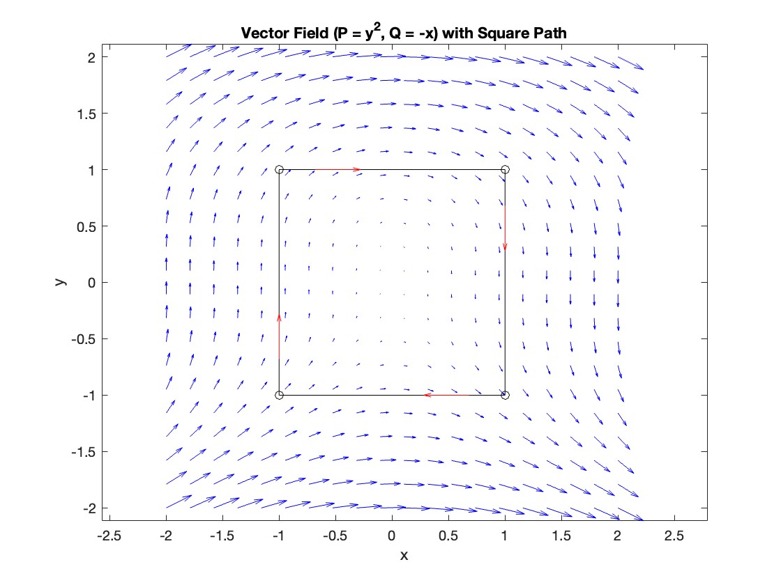
Apply Green's Theorem for the line integral
% Define the partial derivatives of P and Q
f = @(x, y) -1 - 2*y; % derivative of -x with respect to x is -1, and derivative of y^2 with respect to y is 2y
% Compute the double integral over the square [-1,1]x[-1,1]
integral_value = integral2(f, -1, 1, 1, -1);
disp(['Green''s Theorem Integral: ', num2str(integral_value)]);
Plotting the vector field related to Green’s theorem
% Define the grid for the vector field
[x, y] = meshgrid(linspace(-2, 2, 20), linspace(-2 ,2, 20));
% Define the vector field components
P = y.^2; % y^2 component
Q = -x; % -x component
% Plot the vector field
figure;
quiver(x, y, P, Q, 'b');
hold on; % Hold on to plot the square on the same figure
% Define the square's vertices
vertices = [-1 -1; -1 1; 1 1; 1 -1; -1 -1];
% Plot the square path
plot(vertices(:,1), vertices(:,2), '-o', 'Color', 'k'); % 'k' for black color
title('Vector Field (P = y^2, Q = -x) with Square Path');
xlabel('x');
ylabel('y');
axis equal;
% Add arrows to indicate the path direction (counterclockwise)
for i = 1:size(vertices,1)-1
% Calculate direction
dx = vertices(i+1,1) - vertices(i,1);
dy = vertices(i+1,2) - vertices(i,2);
% Reduce the length of the arrow for better visibility
scale = 0.2;
dx = scale * dx;
dy = scale * dy;
% Calculate the start point of the arrow
startx = vertices(i,1) + (1 - scale) * dx;
starty = vertices(i,2) + (1 - scale) * dy;
% Plot the arrow
quiver(startx, starty, dx, dy, 'MaxHeadSize', 0.5, 'Color', 'r', 'AutoScale', 'off');
end
hold off;
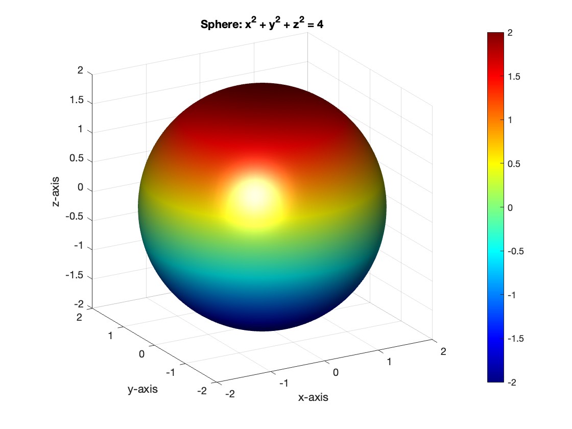
To solve a surface integral for example the over the sphere
  easily in MATLAB, you can leverage the symbolic toolbox for a direct and clear solution. Here is a tip to simplify the process:
over the sphere - Use Symbolic Variables and Functions: Define your variables symbolically, including the parameters of your spherical coordinates θ and ϕ and the radius r . This allows MATLAB to handle the expressions symbolically, making it easier to manipulate and integrate them.
- Express in Spherical Coordinates Directly: Since you already know the sphere's equation and the relationship in spherical coordinates, define x, y, and z in terms of r , θ and ϕ directly.
- Perform Symbolic Integration: Use MATLAB's `int` function to integrate symbolically. Since the sphere and the function
 are symmetric, you can exploit these symmetries to simplify the calculation.
Here’s how you can apply this tip in MATLAB code:
% Include the symbolic math toolbox
syms theta phi
% Define the limits for theta and phi
theta_limits = [0, pi];
phi_limits = [0, 2*pi];
% Define the integrand function symbolically
integrand = 16 * sin(theta)^3 * cos(phi)^2;
% Perform the symbolic integral for the surface integral
surface_integral = int(int(integrand, theta, theta_limits(1), theta_limits(2)), phi, phi_limits(1), phi_limits(2));
% Display the result of the surface integral symbolically
disp(['The surface integral of x^2 over the sphere is ', char(surface_integral)]);
% Number of points for plotting
num_points = 100;
% Define theta and phi for the sphere's surface
[theta_mesh, phi_mesh] = meshgrid(linspace(double(theta_limits(1)), double(theta_limits(2)), num_points), ...
linspace(double(phi_limits(1)), double(phi_limits(2)), num_points));
% Spherical to Cartesian conversion for plotting
r = 2; % radius of the sphere
x = r * sin(theta_mesh) .* cos(phi_mesh);
y = r * sin(theta_mesh) .* sin(phi_mesh);
z = r * cos(theta_mesh);
% Plot the sphere
figure;
surf(x, y, z, 'FaceColor', 'interp', 'EdgeColor', 'none');
colormap('jet'); % Color scheme
shading interp; % Smooth shading
camlight headlight; % Add headlight-type lighting
lighting gouraud; % Use Gouraud shading for smooth color transitions
title('Sphere: x^2 + y^2 + z^2 = 4');
xlabel('x-axis');
ylabel('y-axis');
zlabel('z-axis');
colorbar; % Add color bar to indicate height values
axis square; % Maintain aspect ratio to be square
view([-30, 20]); % Set a nice viewing angle
Before we begin, you will need to make sure you have 'sir_age_model.m' installed. Once you've downloaded this folder into your working directory, which can be located at your current folder. If you can see this file in your current folder, then it's safe to use it. If you choose to use MATLAB online or MATLAB Mobile, you may upload this to your MATLAB Drive.
This is the code for the SIR model stratified into 2 age groups (children and adults). For a detailed explanation of how to derive the force of infection by age group.
% Main script to run the SIR model simulation
% Initial state values
initial_state_values = [200000; 1; 0; 800000; 0; 0]; % [S1; I1; R1; S2; I2; R2]
% Parameters
parameters = [0.05; 7; 6; 1; 10; 1/5]; % [b; c_11; c_12; c_21; c_22; gamma]
% Time span for the simulation (3 months, with daily steps)
tspan = [0 90];
% Solve the ODE
[t, y] = ode45(@(t, y) sir_age_model(t, y, parameters), tspan, initial_state_values);
% Plotting the results
plot(t, y);
xlabel('Time (days)');
ylabel('Number of people');
legend('S1', 'I1', 'R1', 'S2', 'I2', 'R2');
title('SIR Model with Age Structure');
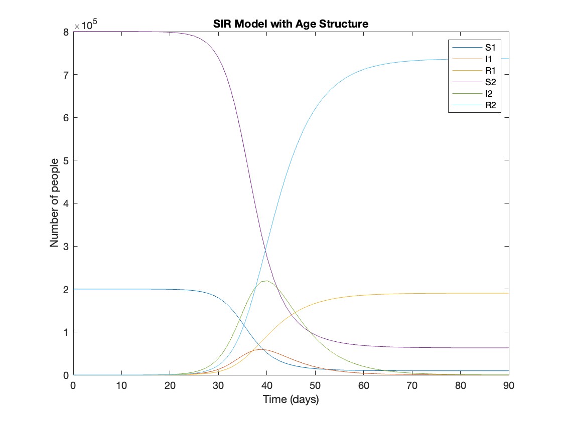
What was the cumulative incidence of infection during this epidemic? What proportion of those infections occurred in children?
In the SIR model, the cumulative incidence of infection is simply the decline in susceptibility.
% Assuming 'y' contains the simulation results from the ode45 function
% and 't' contains the time points
% Total cumulative incidence
total_cumulative_incidence = (y(1,1) - y(end,1)) + (y(1,4) - y(end,4));
fprintf('Total cumulative incidence: %f\n', total_cumulative_incidence);
% Cumulative incidence in children
cumulative_incidence_children = (y(1,1) - y(end,1));
% Proportion of infections in children
proportion_infections_children = cumulative_incidence_children / total_cumulative_incidence;
fprintf('Proportion of infections in children: %f\n', proportion_infections_children);
927,447 people became infected during this epidemic, 20.5% of which were children.
Which age group was most affected by the epidemic?
To answer this, we can calculate the proportion of children and adults that became infected.
% Assuming 'y' contains the simulation results from the ode45 function
% and 't' contains the time points
% Proportion of children that became infected
initial_children = 200000; % initial number of susceptible children
final_susceptible_children = y(end,1); % final number of susceptible children
proportion_infected_children = (initial_children - final_susceptible_children) / initial_children;
fprintf('Proportion of children that became infected: %f\n', proportion_infected_children);
% Proportion of adults that became infected
initial_adults = 800000; % initial number of susceptible adults
final_susceptible_adults = y(end,4); % final number of susceptible adults
proportion_infected_adults = (initial_adults - final_susceptible_adults) / initial_adults;
fprintf('Proportion of adults that became infected: %f\n', proportion_infected_adults);
Throughout this epidemic, 95% of all children and 92% of all adults were infected. Children were therefore slightly more affected in proportion to their population size, even though the majority of infections occurred in adults.
I would like to propose the creation of MATLAB EduHub, a dedicated channel within the MathWorks community where educators, students, and professionals can share and access a wealth of educational material that utilizes MATLAB. This platform would act as a central repository for articles, teaching notes, and interactive learning modules that integrate MATLAB into the teaching and learning of various scientific fields.
Key Features:
1. Resource Sharing: Users will be able to upload and share their own educational materials, such as articles, tutorials, code snippets, and datasets.
2. Categorization and Search: Materials can be categorized for easy searching by subject area, difficulty level, and MATLAB version..
3. Community Engagement: Features for comments, ratings, and discussions to encourage community interaction.
4. Support for Educators: Special sections for educators to share teaching materials and track engagement.
Benefits:
- Enhanced Educational Experience: The platform will enrich the learning experience through access to quality materials.
- Collaboration and Networking: It will promote collaboration and networking within the MATLAB community.
- Accessibility of Resources: It will make educational materials available to a wider audience.
By establishing MATLAB EduHub, I propose a space where knowledge and experience can be freely shared, enhancing the educational process and the MATLAB community as a whole.
We have created a new distance learning community for educators who are teaching remotely or online using MathWorks tools. It houses resources, such as articles, code examples, and videos, as well as an area where community members can ask questions or hold discussions around best practices in distance learning. Jiro Doke , who also writes for the File Exchange Pick of the Week blog, will be moderating this community.
We encourage you to visit the new community and share best practices, examples, and ask questions.