Contenu principal

Résultats pour

Educators in mid 2025 worried about students asking an AI to write their required research paper. Now, with agentic AI, students can open their LMS with say Comet and issue the prompt “Hey, complete all my assignments in all of my courses. Thanks!” Done. Thwarting illegitimate use of AIs in education without hindering the many legitimate uses is a cat-and-mouse game and burgeoning industry.
I am actually more interested in a new AI-related teaching and learning challenge: how one AI can teach another AI. To be specific, I have been discovering with Claude macOS App running Opus 4.5 how to school LM Studio macOS App running a local open model Qwen2.5 32B in the use of MATLAB and other MCP services available to both apps, so, like Claude, LM Studio can operate all of my MacOS apps, including regular (Safari) and agentic (Comet or Chrome with Claude Chrome Extension) browsers and other AI Apps like ChatGPT or Perplexity, and can write and debug MATLAB code agentically. (Model Context Protocol is the standardized way AI apps communicate with tools.) You might be playing around with multiple AIs and encountering similar issues. I expect the AI-to-AI teaching and learning challenge to go far beyond my little laptop milieu.
To make this concrete, I offer the image below, which shows LM Studio creating its first Excel spreadsheet using Excel macOS app. Claude App in the left is behind the scenes there updating LM Studio's context window.
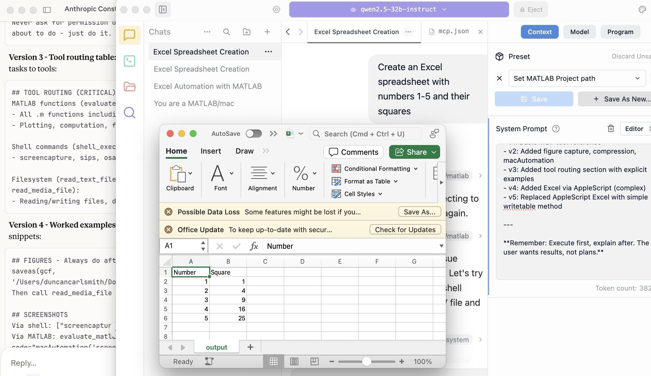
A teacher needs to know something but is at best a guide and inspiration, never a total fount of knowedge, especially today. Working first with Claude alone over the last few weeks to develop skills has itself been an interesting collaborative teaching and learning experience. We had to figure out how to use our MATLAB and other MCP services with various macOS services and some ancillary helper MATLAB functions with hopefully the minimal macOS permissions needed to achieve the desired functionality. Loose permissions allow the AI to access a wider filesystem with shell access, and, for example, to read or even modify an application’s preferences and permissions, and to read its state variables and log files. This is valuable information to an AI in trying to successfully operate an application to achieve some goal. But one might not be comfortable being too permissive.
The result of this collaboration was an expanding bag of tricks: Use AppleScript for this app, but a custom Apple shortcut for this other app; use MATLAB image compression of a screenshot (to provide feedback on the state and results) here, but if MATLAB is not available, then another slower image processing application; use cliclick if an application exposes its UI elements to the Accessibility API, but estimate a cursor relocation from a screenshot of one or more application windows otherwise. Texting images as opposed to text (MMS v SMS) was a challenge. And it’s going to be more complex if I use a multi-monitor setup.
Having satisfied myself that we could, with dedication, learn to operate any app (though each might offer new challenges), I turned to training another AI, similarly empowered with MCP services, to do the same, and that became an interesting new challenge. Firstly, we struggled with the Perplexity App, configured with identical MCP and other services, and found that Perplexity seems unable to avail itself of them. So we turned to educating LM Studio, operating a suite of models downloaded to my laptop.
An AI today is just a model trained in language prediction at some time. It is task-oriented and doesn’t know what to do in a new environment. It needs direction and context, both general and specific. AI’s now have web access to current web information and, given agentic powers, can on their own ask other AI’s for advice. They are quick-studies.
The first question in educating LM Studio was which open model to use. I wanted one that matched my laptop hardware - an APPLE M1 Max (10-core) CPU with integrated 24-core GPU with 64 GB shared memory- and had smarts comparable to Claude’s Opus 4.5 model. We settled on Mistral-Nemo-Instruct 2407 (12B parameters, ~7GB) and got it to the point where it could write and execute a MATLAB code to numerically integrate the equations of motion for a pendulum. Along the way, delving into the observation that the Mistral model's pendulum amplitude was drifting, I learned from Claude about symplectic integration. A teacher is always learning. Learning makes teaching fun.
But, long story short, we learned in the end that this model in this context was unable to see logical errors in code and fix them like Claude. So we tried and settled on some different models: Qwen 2.5 7B Instruct for speed, or Qwen 2.5 32B Instruct for more complex reasoning. The preliminary results looks good!
Our main goal was to teach a model how to use the unusual MCP and linked services at its disposal, starting from zero, and as you might educate a beginning student in physics or whatever through exercises and direct experience. Along the way, in teaching for the first time, we developed a kind of nascent curriculum strategy just to introduce the model to its new capabilities. Allow me to let Claude summarize just to give you a sense. There will not be a test on this material.
The Bootstrapping Process
Phase 1: Discovery of the Problem
The Qwen/Mistral models would describe what they would do rather than execute tools. They'd output JSON text showing what a tool call would look like, rather than actually triggering the tool. Or they'd say "I would use the evaluate_matlab_code tool to..." without doing it.
Phase 2: Explicit Tool Naming
First fix - be explicit in prompts:
Use the evaluate_matlab_code tool to run this code...
Instead of:
Run this MATLAB script...
This worked, but required the user to know tool names.
Phase 3: System Prompt Engineering
We iteratively built up a system prompt (Context tab in LM Studio) that taught the model:
Version 1 - Basic path:
When using MATLAB tools, always use /Users/username/Documents/MATLAB
as the project_path unless the user specifies otherwise.
Version 2 - Forceful execution:
IMPORTANT: When you need to use a tool, execute it immediately.
Do not describe the tool call or show JSON - just call the tool directly.
Never ask for permission or explain what you're about to do - just do it.
Version 3 - Tool routing table:
Added explicit mapping of tasks to tools:
## TOOL ROUTING (CRITICAL)
MATLAB functions (evaluate_matlab_code):
- All .m functions including macAutomation()
- Plotting, computation, file I/O
Shell commands (shell_execute):
- screencapture, sips, osascript, open, say...
Filesystem (read_text_file, write_file, read_media_file):
- Reading/writing files, displaying images
Version 4 - Worked examples:
Added concrete code snippets:
## FIGURES - Always do after plotting:
saveas(gcf, '/Users/username/Documents/MATLAB/LMStudio/latest_figure.png');
Then call read_media_file to display it.
## SCREENSHOTS
Via shell: ["screencapture", "-x", "output.png"]
Via MATLAB: evaluate_matlab_code with code="macAutomation('screenshot','screen')"
Version 5 - Physics patterns:
## PHYSICS - Use Symplectic Integration
omega(i) = omega(i-1) - (g/L)*sin(theta(i-1))*dt;
theta(i) = theta(i-1) + omega(i)*dt; % Use NEW omega
NOT: theta(i-1) + omega(i-1)*dt % Forward Euler drifts!
Phase 4: Prompt Phrasing for Smaller Models
Discovered that 7B-12B models needed "forceful" phrasing:
Execute now: Use evaluate_matlab_code to run this code...
And recovery prompts when they stalled:
Proceed with the tool call
Execute the fix now
Phase 5: Saving as Preset
Along the way, we accumulated various AI-speak directions and ultimately the whole context as a Preset in LM Studio, so it persists across sessions.
Now the trend in the AI industry is to develop and then share or publish “skills” rather like the Preset in a standard markdown structure, like CliffsNotes for AI. My notes/skills won't fit your environment and are evolving. They may appear biased against French models and too pro-Anthropic, and so on. We may need to structure AI education and AI specialization going forward in innovative ways, but may face familiar issues. Some AIs can be self-taught given the slightest nudge. Others less resource priviledged will struggle in their education and future careers. Some may even try to cheat and face a comeuppance.
The next step is to see if Claude can delegate complex tasks to local models, creating a tiered system where a frontier model orchestrates while cheaper models execute.
This project discusses predator-prey system, particularly the Lotka-Volterra equations,which model the interaction between two sprecies: prey and predators. Let's solve the Lotka-Volterra equations numerically and visualize the results.% Define parameters
% Define parameters
alpha = 1.0; % Prey birth rate
beta = 0.1; % Predator success rate
gamma = 1.5; % Predator death rate
delta = 0.075; % Predator reproduction rate
% Define the symbolic variables
syms R W
% Define the equations
eq1 = alpha * R - beta * R * W == 0;
eq2 = delta * R * W - gamma * W == 0;
% Solve the equations
equilibriumPoints = solve([eq1, eq2], [R, W]);
% Extract the equilibrium point values
Req = double(equilibriumPoints.R);
Weq = double(equilibriumPoints.W);
% Display the equilibrium points
equilibriumPointsValues = [Req, Weq]
equilibriumPointsValues = 2x2
0 0 20 10
<mw-icon class=""></mw-icon>
% Solve the differential equations using ode45
lotkaVolterra = @(t,Y)[alpha*Y(1)-beta*Y(1)*Y(2);
delta*Y(1)*Y(2)-gamma*Y(2)];
% Initial conditions
R0 = 40;
W0 = 9;
Y0 = [R0, W0];
tspan = [0, 100];
% Solve the differential equations
[t, Y] = ode45(lotkaVolterra, tspan, Y0);
% Extract the populations
R = Y(:, 1);
W = Y(:, 2);
% Plot the results
figure;
subplot(2,1,1);
plot(t, R, 'r', 'LineWidth', 1.5);
hold on;
plot(t, W, 'b', 'LineWidth', 1.5);
xlabel('Time (months)');
ylabel('Population');
legend('R', 'W');
grid on;
subplot(2,1,2);
plot(R, W, 'k', 'LineWidth', 1.5);
xlabel('R');
ylabel('W');
grid on;
hold on;
plot(Req, Weq, 'ro', 'MarkerSize', 8, 'MarkerFaceColor', 'r');
legend('Phase Trajectory', 'Equilibrium Point');
Now, we need to handle a modified version of the Lotka-Volterra equations. These modified equations incorporate logistic growth fot the prey population.
These equations are:
% Define parameters
alpha = 1.0;
K = 100; % Carrying Capacity of the prey population
beta = 0.1;
gamma = 1.5;
delta = 0.075;
% Define the symbolic variables
syms R W
% Define the equations
eq1 = alpha*R*(1 - R/K) - beta*R*W == 0;
eq2 = delta*R*W - gamma*W == 0;
% Solve the equations
equilibriumPoints = solve([eq1, eq2], [R, W]);
% Extract the equilibrium point values
Req = double(equilibriumPoints.R);
Weq = double(equilibriumPoints.W);
% Display the equilibrium points
equilibriumPointsValues = [Req, Weq]
equilibriumPointsValues = 3x2
0 0 20 8 100 0
<mw-icon class=""></mw-icon>
% Solve the differential equations using ode45
modified_lv = @(t,Y)[alpha*Y(1)*(1-Y(1)/K)-beta*Y(1)*Y(2);
delta*Y(1)*Y(2)-gamma*Y(2)];
% Initial conditions
R0 = 40;
W0 = 9;
Y0 = [R0, W0];
tspan = [0, 100];
% Solve the differential equations
[t, Y] = ode45(modified_lv, tspan, Y0);
% Extract the populations
R = Y(:, 1);
W = Y(:, 2);
% Plot the results
figure;
subplot(2,1,1);
plot(t, R, 'r', 'LineWidth', 1.5);
hold on;
plot(t, W, 'b', 'LineWidth', 1.5);
xlabel('Time (months)');
ylabel('Population');
legend('R', 'W');
grid on;
subplot(2,1,2);
plot(R, W, 'k', 'LineWidth', 1.5);
xlabel('R');
ylabel('W');
grid on;
hold on;
plot(Req, Weq, 'ro', 'MarkerSize', 8, 'MarkerFaceColor', 'r');
legend('Phase Trajectory', 'Equilibrium Point');
While searching the internet for some books on ordinary differential equations, I came across a link that I believe is very useful for all math students and not only. If you are interested in ODEs, it's worth taking the time to study it.
A First Look at Ordinary Differential Equations by Timothy S. Judson is an excellent resource for anyone looking to understand ODEs better. Here's a brief overview of the main topics covered:
  1. Introduction to ODEs: Basic concepts, definitions, and initial differential equations.
  2. Methods of Solution:
  • Separable equations
  • First-order linear equations
  • Exact equations
  • Transcendental functions
  1. Applications of ODEs: Practical examples and applications in various scientific fields.
  2. Systems of ODEs: Analysis and solutions of systems of differential equations.
  3. Series and Numerical Methods: Use of series and numerical methods for solving ODEs.
This book provides a clear and comprehensive introduction to ODEs, making it suitable for students and new researchers in mathematics. If you're interested, you can explore the book in more detail here: A First Look at Ordinary Differential Equations.
The study of the dynamics of the discrete Klein - Gordon equation (DKG) with friction is given by the equation :
above equation, W describes the potential function :
The objective of this simulation is to model the dynamics of a segment of DNA under thermal fluctuations with fixed boundaries using a modified discrete Klein-Gordon equation. The model incorporates elasticity, nonlinearity, and damping to provide insights into the mechanical behavior of DNA under various conditions.
% Parameters
numBases = 200; % Number of base pairs, representing a segment of DNA
kappa = 0.1; % Elasticity constant
omegaD = 0.2; % Frequency term
beta = 0.05; % Nonlinearity coefficient
delta = 0.01; % Damping coefficient
  • Position: Random initial perturbations between 0.01 and 0.02 to simulate the thermal fluctuations at the start.
  • Velocity: All bases start from rest, assuming no initial movement except for the thermal perturbations.
% Random initial perturbations to simulate thermal fluctuations
initialPositions = 0.01 + (0.02-0.01).*rand(numBases,1);
initialVelocities = zeros(numBases,1); % Assuming initial rest state
The simulation uses fixed ends to model the DNA segment being anchored at both ends, which is typical in experimental setups for studying DNA mechanics. The equations of motion for each base are derived from a modified discrete Klein-Gordon equation with the inclusion of damping:
% Define the differential equations
dt = 0.05; % Time step
tmax = 50; % Maximum time
tspan = 0:dt:tmax; % Time vector
x = zeros(numBases, length(tspan)); % Displacement matrix
x(:,1) = initialPositions; % Initial positions
% Velocity-Verlet algorithm for numerical integration
for i = 2:length(tspan)
% Compute acceleration for internal bases
acceleration = zeros(numBases,1);
for n = 2:numBases-1
acceleration(n) = kappa * (x(n+1, i-1) - 2 * x(n, i-1) + x(n-1, i-1)) ...
- delta * initialVelocities(n) - omegaD^2 * (x(n, i-1) - beta * x(n, i-1)^3);
end
% positions for internal bases
x(2:numBases-1, i) = x(2:numBases-1, i-1) + dt * initialVelocities(2:numBases-1) ...
+ 0.5 * dt^2 * acceleration(2:numBases-1);
% velocities using new accelerations
newAcceleration = zeros(numBases,1);
for n = 2:numBases-1
newAcceleration(n) = kappa * (x(n+1, i) - 2 * x(n, i) + x(n-1, i)) ...
- delta * initialVelocities(n) - omegaD^2 * (x(n, i) - beta * x(n, i)^3);
end
initialVelocities(2:numBases-1) = initialVelocities(2:numBases-1) + 0.5 * dt * (acceleration(2:numBases-1) + newAcceleration(2:numBases-1));
end
% Visualization of displacement over time for each base pair
figure;
hold on;
for n = 2:numBases-1
plot(tspan, x(n, :));
end
xlabel('Time');
ylabel('Displacement');
legend(arrayfun(@(n) ['Base ' num2str(n)], 2:numBases-1, 'UniformOutput', false));
title('Displacement of DNA Bases Over Time');
hold off;
The results are visualized using a plot that shows the displacements of each base over time . Key observations from the simulation include :
  • Wave Propagation: The initial perturbations lead to wave-like dynamics along the segment, with visible propagation and reflection at the boundaries.
  • Damping Effects: The inclusion of damping leads to a gradual reduction in the amplitude of the oscillations, indicating energy dissipation over time.
  • Nonlinear Behavior: The nonlinear term influences the response, potentially stabilizing the system against large displacements or leading to complex dynamic patterns.
% 3D plot for displacement
figure;
[X, T] = meshgrid(1:numBases, tspan);
surf(X', T', x);
xlabel('Base Pair');
ylabel('Time');
zlabel('Displacement');
title('3D View of DNA Base Displacements');
colormap('jet');
shading interp;
colorbar; % Adds a color bar to indicate displacement magnitude
% Snapshot visualization at a specific time
snapshotTime = 40; % Desired time for the snapshot
[~, snapshotIndex] = min(abs(tspan - snapshotTime)); % Find closest index
snapshotSolution = x(:, snapshotIndex); % Extract displacement at the snapshot time
% Plotting the snapshot
figure;
stem(1:numBases, snapshotSolution, 'filled'); % Discrete plot using stem
title(sprintf('DNA Model Displacement at t = %d seconds', snapshotTime));
xlabel('Base Pair Index');
ylabel('Displacement');
% Time vector for detailed sampling
tDetailed = 0:0.5:50; % Detailed time steps
% Initialize an empty array to hold the data
data = [];
% Generate the data for 3D plotting
for i = 1:numBases
% Interpolate to get detailed solution data for each base pair
detailedSolution = interp1(tspan, x(i, :), tDetailed);
% Concatenate the current base pair's data to the main data array
data = [data; repmat(i, length(tDetailed), 1), tDetailed', detailedSolution'];
end
% 3D Plot
figure;
scatter3(data(:,1), data(:,2), data(:,3), 10, data(:,3), 'filled');
xlabel('Base Pair');
ylabel('Time');
zlabel('Displacement');
title('3D Plot of DNA Base Pair Displacements Over Time');
colorbar; % Adds a color bar to indicate displacement magnitude

Hello MathWorks Community,

I am excited to announce that I am currently working on a book project centered around Matrix Algebra, specifically designed for MATLAB users. This book aims to cater to undergraduate students in engineering, where Matrix Algebra serves as a foundational element.

Matrix Algebra is not only pivotal in understanding complex engineering concepts but also in applying these principles effectively in various technological solutions. MATLAB, renowned for its powerful computational capabilities, is an excellent tool to explore and implement these concepts, making it a perfect companion for this book.

As I embark on this journey to create a resource that bridges theoretical matrix algebra with practical MATLAB applications, I am looking for one or two knowledgeable individuals who have a firm grasp of both subjects. If you have experience in teaching or applying matrix algebra in engineering contexts and are familiar with MATLAB, your contribution could be invaluable.

Collaborators will help in shaping the content to ensure it is educational, engaging, and technically robust, making complex concepts accessible and applicable for students.

If you are interested in contributing to this project or know someone who might be, please reach out to discuss how we can work together to make this book a valuable resource for engineering students.

Thank you and looking forward to your participation!

I'm excited to share some valuable resources that I've found to be incredibly helpful for anyone looking to enhance their MATLAB skills. Whether you're just starting out, studying as a student, or are a seasoned professional, these guides and books offer a wealth of information to aid in your learning journey.
These materials are freely available and can be a great addition to your learning resources. They cover a wide range of topics and are designed to help users at all levels to improve their proficiency in MATLAB.
Happy learning and I hope you find these resources as useful as I have!
The line integral 
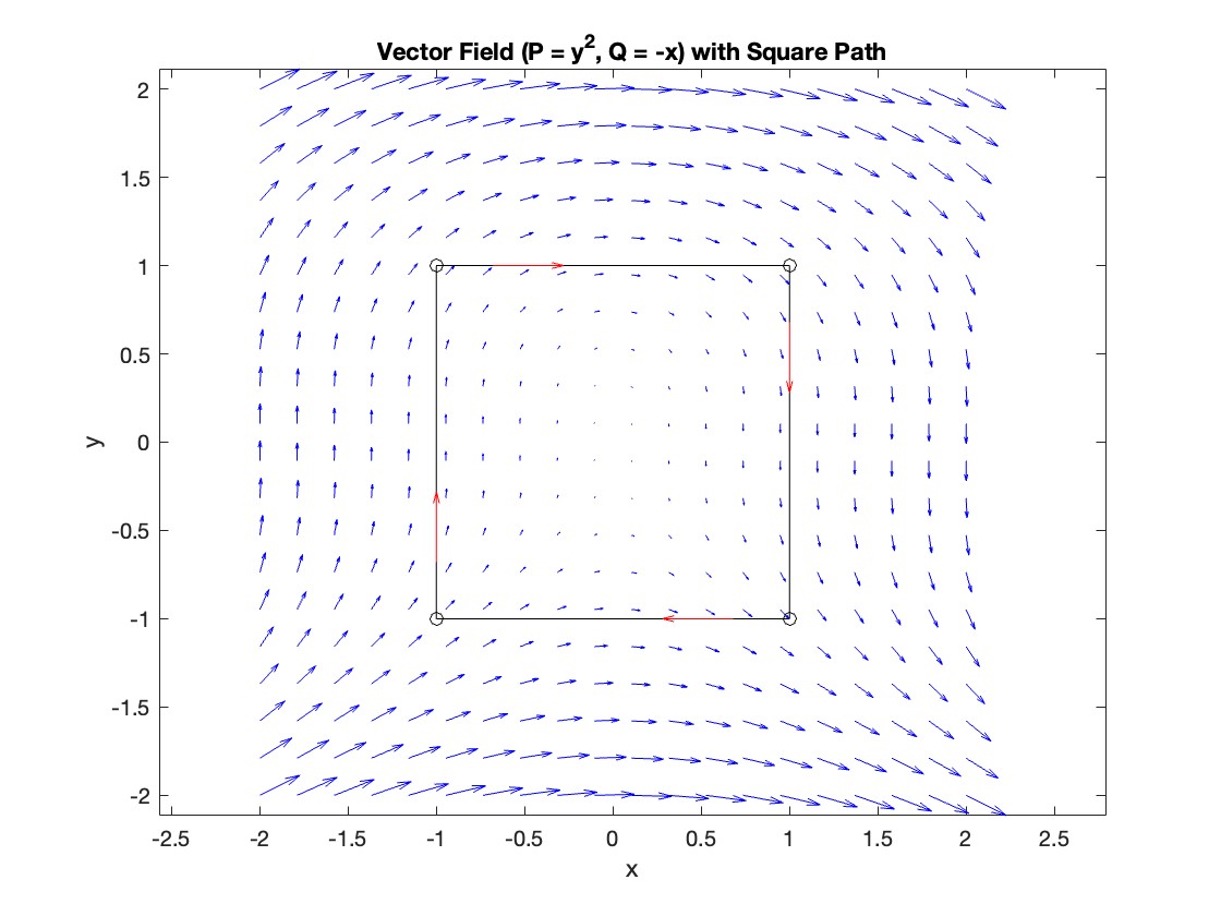
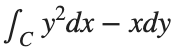
, where C is the boundary of the square
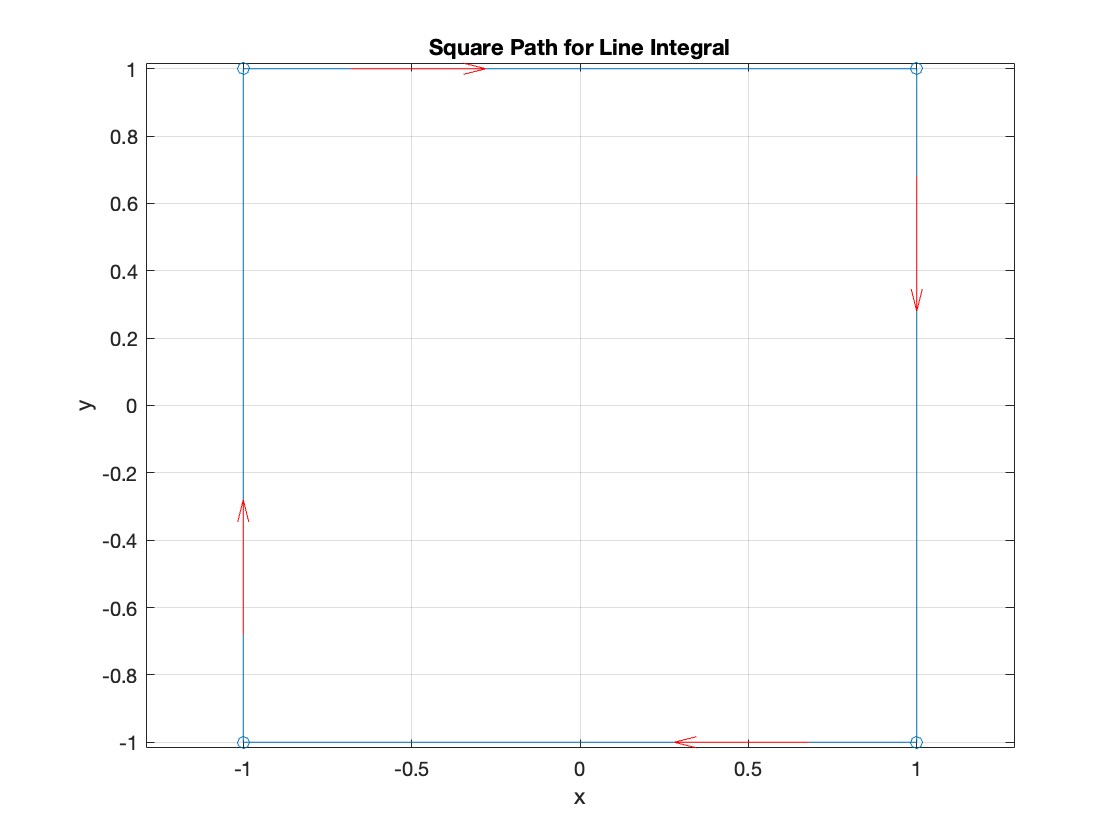
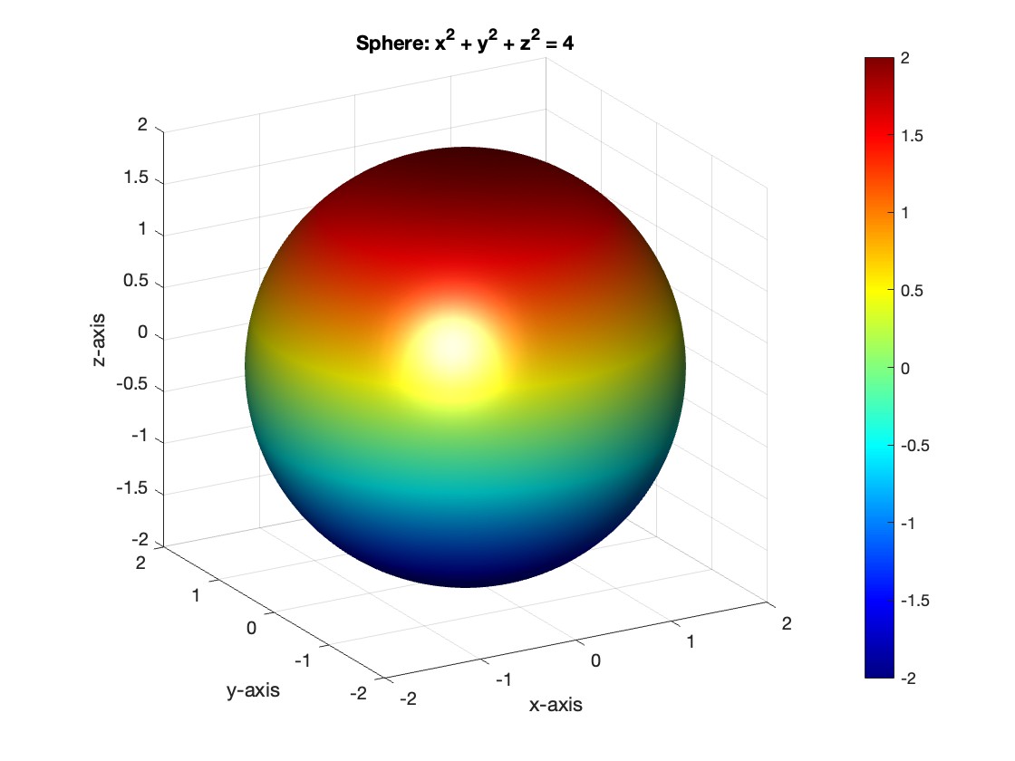
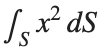
 oriented counterclockwise, can be evaluated in two ways:
Using the definition of the line integral:
% Initialize the integral sum
integral_sum = 0;
% Segment C1: x = -1, y goes from -1 to 1
y = linspace(-1, 1);
x = -1 * ones(size(y));
dy = diff(y);
integral_sum = integral_sum + sum(-x(1:end-1) .* dy);
% Segment C2: y = 1, x goes from -1 to 1
x = linspace(-1, 1);
y = ones(size(x));
dx = diff(x);
integral_sum = integral_sum + sum(y(1:end-1).^2 .* dx);
% Segment C3: x = 1, y goes from 1 to -1
y = linspace(1, -1);
x = ones(size(y));
dy = diff(y);
integral_sum = integral_sum + sum(-x(1:end-1) .* dy);
% Segment C4: y = -1, x goes from 1 to -1
x = linspace(1, -1);
y = -1 * ones(size(x));
dx = diff(x);
integral_sum = integral_sum + sum(y(1:end-1).^2 .* dx);
disp(['Direct Method Integral: ', num2str(integral_sum)]);
Plotting the square path
% Define the square's vertices
vertices = [-1 -1; -1 1; 1 1; 1 -1; -1 -1];
% Plot the square
figure;
plot(vertices(:,1), vertices(:,2), '-o');
title('Square Path for Line Integral');
xlabel('x');
ylabel('y');
grid on;
axis equal;
% Add arrows to indicate the path direction (counterclockwise)
hold on;
for i = 1:size(vertices,1)-1
% Calculate direction
dx = vertices(i+1,1) - vertices(i,1);
dy = vertices(i+1,2) - vertices(i,2);
% Reduce the length of the arrow for better visibility
scale = 0.2;
dx = scale * dx;
dy = scale * dy;
% Calculate the start point of the arrow
startx = vertices(i,1) + (1 - scale) * dx;
starty = vertices(i,2) + (1 - scale) * dy;
% Plot the arrow
quiver(startx, starty, dx, dy, 'MaxHeadSize', 0.5, 'Color', 'r', 'AutoScale', 'off');
end
hold off;
Apply Green's Theorem for the line integral
% Define the partial derivatives of P and Q
f = @(x, y) -1 - 2*y; % derivative of -x with respect to x is -1, and derivative of y^2 with respect to y is 2y
% Compute the double integral over the square [-1,1]x[-1,1]
integral_value = integral2(f, -1, 1, 1, -1);
disp(['Green''s Theorem Integral: ', num2str(integral_value)]);
Plotting the vector field related to Green’s theorem
% Define the grid for the vector field
[x, y] = meshgrid(linspace(-2, 2, 20), linspace(-2 ,2, 20));
% Define the vector field components
P = y.^2; % y^2 component
Q = -x; % -x component
% Plot the vector field
figure;
quiver(x, y, P, Q, 'b');
hold on; % Hold on to plot the square on the same figure
% Define the square's vertices
vertices = [-1 -1; -1 1; 1 1; 1 -1; -1 -1];
% Plot the square path
plot(vertices(:,1), vertices(:,2), '-o', 'Color', 'k'); % 'k' for black color
title('Vector Field (P = y^2, Q = -x) with Square Path');
xlabel('x');
ylabel('y');
axis equal;
% Add arrows to indicate the path direction (counterclockwise)
for i = 1:size(vertices,1)-1
% Calculate direction
dx = vertices(i+1,1) - vertices(i,1);
dy = vertices(i+1,2) - vertices(i,2);
% Reduce the length of the arrow for better visibility
scale = 0.2;
dx = scale * dx;
dy = scale * dy;
% Calculate the start point of the arrow
startx = vertices(i,1) + (1 - scale) * dx;
starty = vertices(i,2) + (1 - scale) * dy;
% Plot the arrow
quiver(startx, starty, dx, dy, 'MaxHeadSize', 0.5, 'Color', 'r', 'AutoScale', 'off');
end
hold off;
To solve a surface integral for example the over the sphere easily in MATLAB, you can leverage the symbolic toolbox for a direct and clear solution. Here is a tip to simplify the process:
  1. Use Symbolic Variables and Functions: Define your variables symbolically, including the parameters of your spherical coordinates θ and ϕ and the radius r . This allows MATLAB to handle the expressions symbolically, making it easier to manipulate and integrate them.
  2. Express in Spherical Coordinates Directly: Since you already know the sphere's equation and the relationship in spherical coordinates, define x, y, and z in terms of r , θ and ϕ directly.
  3. Perform Symbolic Integration: Use MATLAB's `int` function to integrate symbolically. Since the sphere and the function are symmetric, you can exploit these symmetries to simplify the calculation.
Here’s how you can apply this tip in MATLAB code:
% Include the symbolic math toolbox
syms theta phi
% Define the limits for theta and phi
theta_limits = [0, pi];
phi_limits = [0, 2*pi];
% Define the integrand function symbolically
integrand = 16 * sin(theta)^3 * cos(phi)^2;
% Perform the symbolic integral for the surface integral
surface_integral = int(int(integrand, theta, theta_limits(1), theta_limits(2)), phi, phi_limits(1), phi_limits(2));
% Display the result of the surface integral symbolically
disp(['The surface integral of x^2 over the sphere is ', char(surface_integral)]);
% Number of points for plotting
num_points = 100;
% Define theta and phi for the sphere's surface
[theta_mesh, phi_mesh] = meshgrid(linspace(double(theta_limits(1)), double(theta_limits(2)), num_points), ...
linspace(double(phi_limits(1)), double(phi_limits(2)), num_points));
% Spherical to Cartesian conversion for plotting
r = 2; % radius of the sphere
x = r * sin(theta_mesh) .* cos(phi_mesh);
y = r * sin(theta_mesh) .* sin(phi_mesh);
z = r * cos(theta_mesh);
% Plot the sphere
figure;
surf(x, y, z, 'FaceColor', 'interp', 'EdgeColor', 'none');
colormap('jet'); % Color scheme
shading interp; % Smooth shading
camlight headlight; % Add headlight-type lighting
lighting gouraud; % Use Gouraud shading for smooth color transitions
title('Sphere: x^2 + y^2 + z^2 = 4');
xlabel('x-axis');
ylabel('y-axis');
zlabel('z-axis');
colorbar; % Add color bar to indicate height values
axis square; % Maintain aspect ratio to be square
view([-30, 20]); % Set a nice viewing angle
Before we begin, you will need to make sure you have 'sir_age_model.m' installed. Once you've downloaded this folder into your working directory, which can be located at your current folder. If you can see this file in your current folder, then it's safe to use it. If you choose to use MATLAB online or MATLAB Mobile, you may upload this to your MATLAB Drive.
This is the code for the SIR model stratified into 2 age groups (children and adults). For a detailed explanation of how to derive the force of infection by age group.
% Main script to run the SIR model simulation
% Initial state values
initial_state_values = [200000; 1; 0; 800000; 0; 0]; % [S1; I1; R1; S2; I2; R2]
% Parameters
parameters = [0.05; 7; 6; 1; 10; 1/5]; % [b; c_11; c_12; c_21; c_22; gamma]
% Time span for the simulation (3 months, with daily steps)
tspan = [0 90];
% Solve the ODE
[t, y] = ode45(@(t, y) sir_age_model(t, y, parameters), tspan, initial_state_values);
% Plotting the results
plot(t, y);
xlabel('Time (days)');
ylabel('Number of people');
legend('S1', 'I1', 'R1', 'S2', 'I2', 'R2');
title('SIR Model with Age Structure');
What was the cumulative incidence of infection during this epidemic? What proportion of those infections occurred in children?
In the SIR model, the cumulative incidence of infection is simply the decline in susceptibility.
% Assuming 'y' contains the simulation results from the ode45 function
% and 't' contains the time points
% Total cumulative incidence
total_cumulative_incidence = (y(1,1) - y(end,1)) + (y(1,4) - y(end,4));
fprintf('Total cumulative incidence: %f\n', total_cumulative_incidence);
% Cumulative incidence in children
cumulative_incidence_children = (y(1,1) - y(end,1));
% Proportion of infections in children
proportion_infections_children = cumulative_incidence_children / total_cumulative_incidence;
fprintf('Proportion of infections in children: %f\n', proportion_infections_children);
927,447 people became infected during this epidemic, 20.5% of which were children.
Which age group was most affected by the epidemic?
To answer this, we can calculate the proportion of children and adults that became infected.
% Assuming 'y' contains the simulation results from the ode45 function
% and 't' contains the time points
% Proportion of children that became infected
initial_children = 200000; % initial number of susceptible children
final_susceptible_children = y(end,1); % final number of susceptible children
proportion_infected_children = (initial_children - final_susceptible_children) / initial_children;
fprintf('Proportion of children that became infected: %f\n', proportion_infected_children);
% Proportion of adults that became infected
initial_adults = 800000; % initial number of susceptible adults
final_susceptible_adults = y(end,4); % final number of susceptible adults
proportion_infected_adults = (initial_adults - final_susceptible_adults) / initial_adults;
fprintf('Proportion of adults that became infected: %f\n', proportion_infected_adults);
Throughout this epidemic, 95% of all children and 92% of all adults were infected. Children were therefore slightly more affected in proportion to their population size, even though the majority of infections occurred in adults.
goc3
goc3
Dernière activité le 6 Nov 2023

Have you ever learned that something you were doing manually in MATLAB was already possible using a built-in feature? Have you ever written a function only to later realize (or be told) that a built-in function already did what you needed?
Two such moments come to mind for me.
1. Did you realize that you can set conditional breakpoints? Neither did I, until someone showed me that feature. To do that, open or create a file in the editor, right click on a line number for any line that contains code, and select Set Conditional Breakpoint... This will bring up a dialog wherein you can type any logical condition for which execution should be paused. Before I learned about this, I would manually insert if-statements during debugging. Then, after fixing each bug, I would have to delete those statements. This built-in feature is so much better.
2. Have you ever needed to plot horizontal or vertical lines in a plot? For the longest time, I would manually code such lines. Then, I learned about xline() and yline(). Not only is less code required, these lines automatically span the entire axes while zooming, panning, or adjusting axis limits!
Share your own Aha! moments below. This will help everyone learn about MATLAB functionality that may not be obvious or front and center.
(Note: While File Exchange contains many great contributions, the intent of this thread is to focus on built-in MATLAB functionality.)
Exciting news for students! 🚀Simulink Student Challenge 2023 is live! Unleash your engineering skills and compete for exciting rewards. Submission deadline is December 12th, 2023!
Calling all students! New to MATLAB or need helpful resources? Check out our MATLAB GitHub for Students repository! Find MATLAB examples, videos, cheat sheets, and more!
Visit the repository here: MATLAB GitHub for Students

One community within MathWorks that has been helping students continue their learning is MATLAB Student Ambassadors. Despite new challenges with transitioning to distance learning, student ambassadors have done a truly amazing job. In a blog that was published recently, I discuss 3 examples of the great things that our student ambassadors have done to aid distance learning. Click here to read the blog. I hope after reading this blog you share my level of admiration for these students.

Student Ambassador at University of Houston hosting a fun and informative virtual event.