phasedArrayCalculator

R2026b

Create phased array for Gaussian beam analysis

Since R2026b

Description

Use the phasedArrayCalculator object to design and analyze phased array antennas quickly using classical array equations without running full‑wave electromagnetic simulations.

The object lets you:

• Size arrays to meet a target gain

• Explore square and hexagonal lattices

• Evaluate directivity, beamwidth, sidelobe levels, and grating lobes

• Visualize array layout, efficiency trends, and grating lobe angles

• Generate initial 3‑D array models for conformalArray or phased.ConformalArray (Phased Array System Toolbox)

Phased array antennas combine the fields from multiple radiating elements with specified amplitude (taper) and phase distributions to form high‑gain spot beams or shaped coverage beams. Amplitude taper is commonly used to control sidelobe levels, while phase distributions are used to scan or shape the beam. Early‑stage array design via closed‑form array equations is much faster than full‑wave simulation and is useful for initial sizing and trade studies.

Creation

Syntax

Description

p = phasedArrayCalculator creates a 2-by-2 horn-fed parabolic reflector antenna array with default property values.

p = phasedArrayCalculator(PropertyName=Value) sets properties using one or more name-value arguments. PropertyName is the property name and Value is the corresponding value. You can specify several name-value arguments in any order as PropertyName1=Value1,...,PropertyNameN=ValueN. Properties that you do not specify, retain their default values.

For example, p = phasedArrayCalculator(Lattice="hexagon") creates a phased array of horn antennas arranged in a hexagonal lattice with default values for other properties.

Properties

Lattice — Type of arrangement of elements

"square" (default) | "hexagon"

Type of arrangement of elements in the array, specified as one of the following:

• "square" — Square lattice

• "hexagon" — Hexagonal lattice

Example: "hexagon"

Data Types: string

RadiatingElement — Type of radiating element

"horn" (default) | "conicalhorn" | "corrugatedhorn" | "potterhorn" | circularpatch | "rectangularpatch" | "dipole" | "patternfed"

Type of radiating element in the array, specified as one of the following:

• "horn" — A rectangular horn antenna created using the horn object

• "conicalhorn" — A conical horn antenna created using the hornConical object

• "corrugatedhorn" — A corrugated horn antenna created using the hornCorrugated object

• "potterhorn" — A potter horn antenna created using the hornPotter object

• "circularpatch" — A circular microstrip patch antenna created using the patchMicrostripCircular object

• "rectangularpatch" — A rectangular microstrip patch antenna created using the patchMicrostrip object

• "dipole" — A dipole antenna created using the dipole object

• "patternfed" — Pattern data of radiating elements

Example: "patch"

Data Types: string

FileName — Name of radiation pattern data file

[] (default) | character vector | string scalar

Name of the radiation pattern data file with extension, specified as a string or a character vector. You can also specify a full path to the file. This property supports only .txt and .csv files.

On Microsoft^® Windows^® systems, you can use either forward slashes (/) or backslashes (\) as path delimiters, even within the same file name. On UNIX^® and Macintosh systems, use only a / as a delimiter. You can specify this property when you set the RadiatingElement property to "patternfed".

Example: "pattern_data.txt"

Data Types: char | string

ArrayGain — Expected array gain

20 (default) | positive scalar

Expected array gain, specified in dB as a positive scalar greater than 15.

Example: 25

Data Types: double

ElementEfficiency — Element efficiency

100 (default) | positive scalar

Element efficiency, specified as a percentage greater than 10.

Example: 75

Data Types: double

IlluminationTaper — Variation of signal strength

0 (default) | nonnegative scalar

Variation of signal strength across array elements, typically measured from center toward the edges, specified as numeric scalar in dB.

Example: 0.5

Data Types: double

ScanAngle — Beam scan angle

6 (default) | positive scalar

Beam scan angle for the array, specified in degrees as a positive scalar in the range (0, 90).

Example: 45

Data Types: double

TaperLoss — Gain reduction due to applied amplitude tapering

0 (default) | nonnegative scalar

Gain reduction due to applied amplitude tapering across the array elements, specified as a nonnegative scalar in dB.

Example: 0.5

Data Types: double

AntennaLoss — Total antenna system loss

0 (default) | nonnegative scalar

Total antenna system loss, specified as a nonnegative scalar in dB. Total antenna system loss is the sum of all front-end losses between the antenna aperture and the amplifiers, including mismatch, polarization, and insertion losses.

Example: 1

Data Types: double

PointingErrorLoss — Gain reduction due to deviation in beam direction

0 (default) | nonnegative scalar

Gain reduction due to deviation in intended and actual beam direction, specified as a nonnegative scalar in dB.

Example: 0.1

Data Types: double

BeamDiameterLoss — Gain reduction due to finite main beam width

0 (default) | nonnegative scalar

Gain reduction due to the finite main beam width, specified as a nonnegative scalar in dB. The finite main beam width causes gain to decrease toward the edges of the beam relative to the boresight.

Example: 0.5

Data Types: double

ImplementationMargin — Design buffer to account for nonlinearities

0 (default) | nonnegative scalar

Design buffer to account for nonlinearities in the antenna system, specified as a nonnegative scalar in dB. ImplementationMargin represents aggregate performance degradation due to hardware nonidealities such as amplifier compression, phase and amplitude errors, and RF chain nonlinearities.

Example: 1

Data Types: double

Object Functions

createArray	Create conformal array from calculated array design parameters
plot	Visualize phased array layout and plot grating lobes, and efficiency
plotDirectivity	Plot directivity of phased array
removeElements	Remove array elements for better sizing
solve	Compute phased array design parameters

Examples

Create, Size, and Visualize Hexagonal Phased Array of Horn Antennas

Define the target parameters for a hexagonal phased array of horn antennas.

p = phasedArrayCalculator(Lattice="hexagon",...
    ArrayGain=25,...
    ElementEfficiency=90,...
    TaperLoss=0.5,...
    ScanAngle=10,...
    AntennaLoss=1,...
    ImplementationMargin=1)

p = 
  phasedArrayCalculator with properties:

                 Lattice: 'hexagon'
        RadiatingElement: 'horn'
               ArrayGain: 25
       ElementEfficiency: 90
       IlluminationTaper: 0
               ScanAngle: 10
               TaperLoss: 0.5000
             AntennaLoss: 1
       PointingErrorLoss: 0
        BeamDiameterLoss: 0
    ImplementationMargin: 1

Calculate the phased array design parameters at 15 GHz.

solve(p,15e9);

Here is the antenna array design data:
                       INPUT DATA                    
    _________________________________________________

                                                     
                                                _____
                                                     
    Wavelength (mm)                             19.99
    Maximum Scan Angle (°)                         10
    Assumed Grating Lobe Location (°)           19.89
    Desired Max Gain (dBi)                         25
    Required Peak Directivity (dBi)              27.5
    Required Directivity at scan angle (dBi)    29.18
    Array Efficiency (%)                          100

                                DESIGN DATA                            
    ___________________________________________________________________

                                                        Hexagon Lattice
                                                        _______________
                                                                       
    Element Spacing (mm)                                     44.91     
    Element Directivity (dBi)                                17.57     
    Number of Elements                                          17     
    Peak Directivity (dBi)                                   29.87     
    Directivity at 10° (dBi)                                 27.63     
    Half Power Beamwidth (°)                                  6.54     
    Grating Lobe Location relative to Boresight (°)          30.93     
    Grating Lobe Location relative to Scan Angle (°)         19.89     

                          SIDE LOBE DATA                       
    ___________________________________________________________

                                                Hexagon Lattice
                                                _______________
                                                               
    Square Aperture: Sidelobe Location (°)             7.4     
    Square Aperture: Sidelobe Level (dBi)           -13.26     
    Circular Aperture: Sidelobe Location (°)           8.3     
    Circular Aperture: Sidelobe Level (dBi)         -17.57     

Plot the array layout.

figure
plot(p,Type="layout",Frequency=15e9);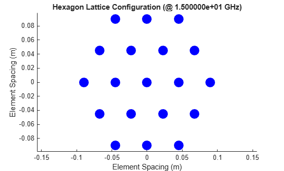

Analyze Phased Array Using Radiation Pattern Data

Create a phasedArrayCalculator object and set the RadiatingElement property to "patternfed". This enables you to use radiation pattern data from a file instead of a predefined element type.

Use the FileName property to specify the radiation pattern data file. Set the array gain and scan angle.

p = phasedArrayCalculator(RadiatingElement="patternfed",...
    FileName="corrugated_horn_12ghz_pattern_data.txt",...
    ArrayGain=25,...
    ScanAngle=6)

p = 
  phasedArrayCalculator with properties:

                 Lattice: 'square'
        RadiatingElement: 'patternfed'
                FileName: "corrugated_horn_12ghz_pattern_data.txt"
               ArrayGain: 25
       ElementEfficiency: 100
       IlluminationTaper: 0
               ScanAngle: 6
               TaperLoss: 0
             AntennaLoss: 0
       PointingErrorLoss: 0
        BeamDiameterLoss: 0
    ImplementationMargin: 0

Use the solve function to compute the design and sidelobe data, and display the input data for the array at 12 GHz.

solve(p,12e9)

Here is the antenna array design data:
                       INPUT DATA                    
    _________________________________________________

                                                     
                                                _____
                                                     
    Wavelength (mm)                             24.98
    Maximum Scan Angle (°)                          6
    Assumed Grating Lobe Location (°)           37.37
    Desired Max Gain (dBi)                         25
    Required Peak Directivity (dBi)                25
    Required Directivity at scan angle (dBi)    26.07
    Array Efficiency (%)                          100

                               DESIGN DATA                            
    __________________________________________________________________

                                                        Square Lattice
                                                        ______________
                                                                      
    Element Spacing (mm)                                    35.12     
    Element Directivity (dBi)                               19.48     
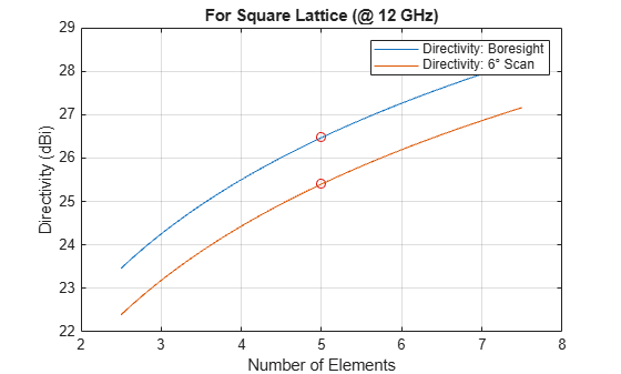
    Number of Elements                                          5     
    Peak Directivity (dBi)                                  26.47     
    Directivity at 6° (dBi)                                  25.4     
    Half Power Beamwidth (°)                                20.84     
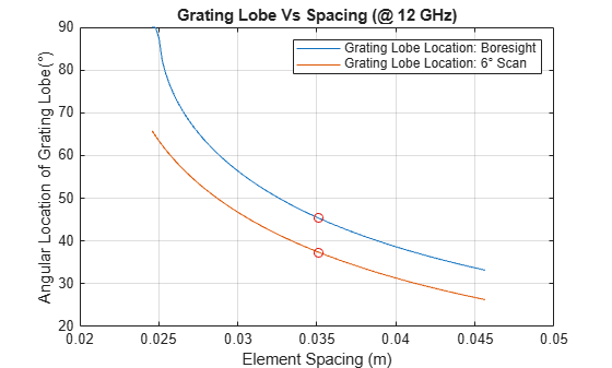
    Grating Lobe Location relative to Boresight (°)         45.35     
    Grating Lobe Location relative to Scan Angle (°)        37.37     

                          SIDE LOBE DATA                      
    __________________________________________________________

                                                Square Lattice
                                                ______________
                                                              
    Square Aperture: Sidelobe Location (°)            19.5    
    Square Aperture: Sidelobe Level (dBi)           -13.26    
    Circular Aperture: Sidelobe Location (°)          22.7    
    Circular Aperture: Sidelobe Level (dBi)         -17.57    

Plot the grating lobe diagram to identify potential grating lobes at 12 GHz operating frequency.

figure
plot(p,Frequency=12e9,Type="gratinglobe")
grid on

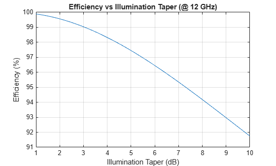
Visualize the array efficiency as a function of illumination taper.

figure
plot(p,Frequency=12e9,Type="efficiency")
grid on

Plot the directivity of the phased array as a function of the number of elements.

figure
plotDirectivity(p,Frequency=12e9,Type="elements")
grid on

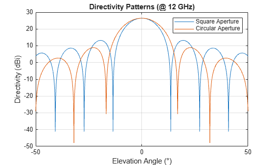
Plot the directivity of the phased array as a function of the elevation angle.

figure
plotDirectivity(p,Frequency=12e9,Type="patterns")
grid on

References

[1] Rao, Sudhakar K., and Calen Ostroot. “Design Principles and Guidelines for Phased Array and Reflector Antennas [Antenna Applications Corner].” IEEE Antennas and Propagation Magazine 62, no. 2 (2020): 74–81. https://doi.org/10.1109/MAP.2020.2969261.

[2] Rao, Sudhakar, Lotfollah Shafai, and Satish Sharma, eds. Handbook of Reflector Antennas and Feed Systems: Volume 3: Applications of Reflectors. Artech House Antennas and Propagation Series. Artech House, 2013.

Version History

Introduced in R2026b