Main Content

make2DOF

Convert 1-DOF PID controller to 2-DOF controller

Description

example

C2 = make2DOF(C1) converts the one-degree-of-freedom PID controller C1 to two degrees of freedom. The setpoint weights b and c of the 2-DOF controller are 1, and the remaining PID coefficients do not change.

C2 = make2DOF(C1,b) specifies the setpoint weight for the proportional term.

example

C2 = make2DOF(C1,b,c) specifies the setpoint weights for both the proportional and derivative terms.

Examples

collapse all

Design a 1-DOF PID controller for a plant.

G = tf(1,[1 0.5 0.1]);
C1 = pidtune(G,'pidf',1.5)
C1 =
 
             1            s    
  Kp + Ki * --- + Kd * --------
             s          Tf*s+1 

  with Kp = 1.12, Ki = 0.23, Kd = 1.3, Tf = 0.122
 
Continuous-time PIDF controller in parallel form.

Convert the controller to two degrees of freedom.

C2 = make2DOF(C1)
C2 =
 
                       1                s    
  u = Kp (b*r-y) + Ki --- (r-y) + Kd -------- (c*r-y)
                       s              Tf*s+1 

  with Kp = 1.12, Ki = 0.23, Kd = 1.3, Tf = 0.122, b = 1, c = 1
 
Continuous-time 2-DOF PIDF controller in parallel form.

The new controller has the same PID gains and filter constant. It also contains new terms involving the setpoint weights b and c. By default, b = c = 1. Therefore, in a closed loop with the plant G, the 2-DOF controller C2 yields the same response as C1.

T1 = feedback(G*C1,1);
CM = tf(C2);
T2 = CM(1)*feedback(G,-CM(2));
stepplot(T1,T2,'r--')

Figure contains an axes object. The axes object contains 2 objects of type line. These objects represent T1, T2.

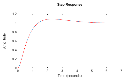
Convert C1 to a 2-DOF controller with different b and c values.

C2_2 = make2DOF(C1,0.5,0.75)
C2_2 =
 
                       1                s    
  u = Kp (b*r-y) + Ki --- (r-y) + Kd -------- (c*r-y)
                       s              Tf*s+1 

  with Kp = 1.12, Ki = 0.23, Kd = 1.3, Tf = 0.122, b = 0.5, c = 0.75
 
Continuous-time 2-DOF PIDF controller in parallel form.

The PID gains and filter constant are still unchanged, but the setpoint weights now change the closed-loop response.

CM_2 = tf(C2_2);
T2_2 = CM_2(1)*feedback(G,-CM_2(2));
stepplot(T1,T2_2,'r--')
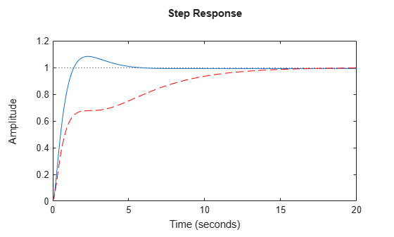
Figure contains an axes object. The axes object contains 2 objects of type line. These objects represent T1, T2\_2.

Input Arguments

collapse all

1-DOF PID controller, specified as a pid object or a pidstd object.

Setpoint weight on proportional term, specified as a real, nonnegative, finite value. If you do not specify b, then C2 has b = 1.

Setpoint weight on derivative term, specified as a real, nonnegative, finite value. If you do not specify c, then C2 has c = 1.

Output Arguments

collapse all

2-DOF PID controller, returned as a pid2 object or pidstd2 object. C2 is in parallel form if C1 is in parallel form, and standard form if C1 is in standard form.

For example, suppose C1 is a continuous-time, parallel-form pid controller of the form:

C1=Kp+Kis+KdsTfs+1.

Then C2 is a parallel-form 2-DOF pid2 controller, which has two inputs and one output. The relationship between the inputs, r and y, and the output u of C2 is given by:

u=Kp(bry)+Kis(ry)+KdsTfs+1(cry).

The PID gains Kp, Ki, and Kd, and the filter time constant Tf are unchanged. The setpoint weights b and c are specified by the input arguments b and c, or 1 by default. For more information about 2-DOF PID controllers, see Two-Degree-of-Freedom PID Controllers.

The conversion also preserves the values of the properties Ts, TimeUnit, Sampling Grid, IFormula, and DFormula.

Version History

Introduced in R2015b