gjr

GJR conditional variance time series model

Description

Use gjr to specify a univariate GJR (Glosten, Jagannathan, and Runkle) model. The gjr function returns a gjr object specifying the functional form of a GJR(P,Q) model, and stores its parameter values.

The key components of a gjr model include the:

• GARCH polynomial, which is composed of lagged conditional variances. The degree is denoted by P.

• ARCH polynomial, which is composed of the lagged squared innovations.

• Leverage polynomial, which is composed of lagged squared, negative innovations.

• Maximum of the ARCH and leverage polynomial degrees, denoted by Q.

P is the maximum nonzero lag in the GARCH polynomial, and Q is the maximum nonzero lag in the ARCH and leverage polynomials. Other model components include an innovation mean model offset, a conditional variance model constant, and the innovations distribution.

All coefficients are unknown (NaN values) and estimable unless you specify their values using name-value pair argument syntax. To estimate models containing all or partially unknown parameter values given data, use estimate. For completely specified models (models in which all parameter values are known), simulate or forecast responses using simulate or forecast, respectively.

Creation

Syntax

Mdl = gjr

Mdl = gjr(P,Q)

Mdl = gjr(Name,Value)

Description

Mdl = gjr returns a zero-degree conditional variance gjr object.

Mdl = gjr(P,Q) creates a GJR conditional variance model object (Mdl) with a GARCH polynomial with a degree of P and ARCH and leverage polynomials each with a degree of Q. All polynomials contain all consecutive lags from 1 through their degrees, and all coefficients are NaN values.

This shorthand syntax enables you to create a template in which you specify the polynomial degrees explicitly. The model template is suited for unrestricted parameter estimation, that is, estimation without any parameter equality constraints. However, after you create a model, you can alter property values using dot notation.

Mdl = gjr(Name,Value) sets properties or additional options using name-value pair arguments. Enclose each property name in quotes. For example, 'ARCHLags',[1 4],'ARCH',{0.2 0.3} specifies the two ARCH coefficients in ARCH at lags 1 and 4.

This longhand syntax enables you to create more flexible models.

Input Arguments

The shorthand syntax provides an easy way for you to create model templates that are suitable for unrestricted parameter estimation. For example, to create a GJR(1,2) model containing unknown parameter values, enter:

Mdl = gjr(1,2);

To impose equality constraints on parameter values during estimation, set the appropriate property values using dot notation.

P — GARCH polynomial degree

nonnegative integer

GARCH polynomial degree, specified as a nonnegative integer. In the GARCH polynomial and at time t, MATLAB^® includes all consecutive conditional variance terms from lag t – 1 through lag t – P.

You can specify this argument using the gjr(P,Q) shorthand syntax only.

If P > 0, then you must specify Q as a positive integer.

Example: gjr(1,1)

Data Types: double

Q — ARCH polynomial degree

nonnegative integer

ARCH polynomial degree, specified as a nonnegative integer. In the ARCH polynomial and at time t, MATLAB includes all consecutive squared innovation terms (for the ARCH polynomial) and squared, negative innovation terms (for the leverage polynomial) from lag t – 1 through lag t – Q.

You can specify this argument using the gjr(P,Q) shorthand syntax only.

If P > 0, then you must specify Q as a positive integer.

Example: gjr(1,1)

Data Types: double

Name-Value Arguments

Specify optional pairs of arguments as Name1=Value1,...,NameN=ValueN, where Name is the argument name and Value is the corresponding value. Name-value arguments must appear after other arguments, but the order of the pairs does not matter.

Before R2021a, use commas to separate each name and value, and enclose Name in quotes.

The longhand syntax enables you to create models in which some or all coefficients are known. During estimation, estimate imposes equality constraints on any known parameters.

Example: 'ARCHLags',[1 4],'ARCH',{NaN NaN} specifies a GJR(0,4) model and unknown, but nonzero, ARCH coefficient matrices at lags 1 and 4.

GARCHLags — GARCH polynomial lags

1:P (default) | numeric vector of unique positive integers

GARCH polynomial lags, specified as the comma-separated pair consisting of 'GARCHLags' and a numeric vector of unique positive integers.

GARCHLags(j) is the lag corresponding to the coefficient GARCH{j}. The lengths of GARCHLags and GARCH must be equal.

Assuming all GARCH coefficients (specified by the GARCH property) are positive or NaN values, max(GARCHLags) determines the value of the P property.

Example: 'GARCHLags',[1 4]

Data Types: double

ARCHLags — ARCH polynomial lags

1:Q (default) | numeric vector of unique positive integers

ARCH polynomial lags, specified as the comma-separated pair consisting of 'ARCHLags' and a numeric vector of unique positive integers.

ARCHLags(j) is the lag corresponding to the coefficient ARCH{j}. The lengths of ARCHLags and ARCH must be equal.

Assuming all ARCH and leverage coefficients (specified by the ARCH and Leverage properties) are positive or NaN values, max([ARCHLags LeverageLags]) determines the value of the Q property.

Example: 'ARCHLags',[1 4]

Data Types: double

LeverageLags — Leverage polynomial lags

1:Q (default) | numeric vector of unique positive integers

Leverage polynomial lags, specified as the comma-separated pair consisting of 'LeverageLags' and a numeric vector of unique positive integers.

LeverageLags(j) is the lag corresponding to the coefficient Leverage{j}. The lengths of LeverageLags and Leverage must be equal.

Assuming all ARCH and leverage coefficients (specified by the ARCH and Leverage properties) are positive or NaN values, max([ARCHLags LeverageLags]) determines the value of the Q property.

Example: 'LeverageLags',1:4

Data Types: double

Properties

You can set writable property values when you create the model object by using name-value pair argument syntax, or after you create the model object by using dot notation. For example, to create a GJR(1,1) model with unknown coefficients, and then specify a t innovation distribution with unknown degrees of freedom, enter:

Mdl = gjr('GARCHLags',1,'ARCHLags',1);
Mdl.Distribution = "t";

P — GARCH polynomial degree

nonnegative integer

This property is read-only.

GARCH polynomial degree, specified as a nonnegative integer. P is the maximum lag in the GARCH polynomial with a coefficient that is positive or NaN. Lags that are less than P can have coefficients equal to 0.

P specifies the minimum number of presample conditional variances required to initialize the model.

If you use name-value pair arguments to create the model, then MATLAB implements one of these alternatives (assuming the coefficient of the largest lag is positive or NaN):

• If you specify GARCHLags, then P is the largest specified lag.

• If you specify GARCH, then P is the number of elements of the specified value. If you also specify GARCHLags, then gjr uses GARCHLags to determine P instead.

• Otherwise, P is 0.

Data Types: double

Q — Maximum degree of ARCH and leverage polynomials

nonnegative integer

This property is read-only.

Maximum degree of ARCH and leverage polynomials, specified as a nonnegative integer. Q is the maximum lag in the ARCH and leverage polynomials in the model. In either type of polynomial, lags that are less than Q can have coefficients equal to 0.

Q specifies the minimum number of presample innovations required to initiate the model.

If you use name-value pair arguments to create the model, then MATLAB implements one of these alternatives (assuming the coefficients of the largest lags in the ARCH and leverage polynomials are positive or NaN):

• If you specify ARCHLags or LeverageLags, then Q is the maximum between the two specifications.

• If you specify ARCH or Leverage, then Q is the maximum number of elements between the two specifications. If you also specify ARCHLags or LeverageLags, then gjr uses their values to determine Q instead.

• Otherwise, Q is 0.

Data Types: double

Constant — Conditional variance model constant

NaN (default) | positive scalar

Conditional variance model constant, specified as a positive scalar or NaN value.

Data Types: double

GARCH — GARCH polynomial coefficients

cell vector of positive scalars or NaN values

GARCH polynomial coefficients, specified as a cell vector of positive scalars or NaN values.

• If you specify GARCHLags, then the following conditions apply.

  • The lengths of GARCH and GARCHLags are equal.

  • GARCH{j} is the coefficient of lag GARCHLags(j).

  • By default, GARCH is a numel(GARCHLags)-by-1 cell vector of NaN values.

• Otherwise, the following conditions apply.

  • The length of GARCH is P.

  • GARCH{j} is the coefficient of lag j.

  • By default, GARCH is a P-by-1 cell vector of NaN values.

The coefficients in GARCH correspond to coefficients in an underlying LagOp lag operator polynomial, and are subject to a near-zero tolerance exclusion test. If you set a coefficient to 1e–12 or below, gjr excludes that coefficient and its corresponding lag in GARCHLags from the model.

Data Types: cell

ARCH — ARCH polynomial coefficients

cell vector of positive scalars or NaN values

ARCH polynomial coefficients, specified as a cell vector of positive scalars or NaN values.

• If you specify ARCHLags, then the following conditions apply.

  • The lengths of ARCH and ARCHLags are equal.

  • ARCH{j} is the coefficient of lag ARCHLags(j).

  • By default, ARCH is a Q-by-1 cell vector of NaN values. For more details, see the Q property.

• Otherwise, the following conditions apply.

  • The length of ARCH is Q.

  • ARCH{j} is the coefficient of lag j.

  • By default, ARCH is a Q-by-1 cell vector of NaN values.

The coefficients in ARCH correspond to coefficients in an underlying LagOp lag operator polynomial, and are subject to a near-zero tolerance exclusion test. If you set a coefficient to 1e–12 or below, gjr excludes that coefficient and its corresponding lag in ARCHLags from the model.

Data Types: cell

Leverage — Leverage polynomial coefficients

cell vector of numeric scalars or NaN values

Leverage polynomial coefficients, specified as a cell vector of numeric scalars or NaN values.

• If you specify LeverageLags, then the following conditions apply.

  • The lengths of Leverage and LeverageLags are equal.

  • Leverage{j} is the coefficient of lag LeverageLags(j).

  • By default, Leverage is a Q-by-1 cell vector of NaN values. For more details, see the Q property.

• Otherwise, the following conditions apply.

  • The length of Leverage is Q.

  • Leverage{j} is the coefficient of lag j.

  • By default, Leverage is a Q-by-1 cell vector of NaN values.

The coefficients in Leverage correspond to coefficients in an underlying LagOp lag operator polynomial, and are subject to a near-zero tolerance exclusion test. If you set a coefficient to 1e–12 or below, gjr excludes that coefficient and its corresponding lag in LeverageLags from the model.

Data Types: cell

UnconditionalVariance — Model unconditional variance

positive scalar

This property is read-only.

The model unconditional variance, specified as a positive scalar.

The unconditional variance is

$${\sigma }_{\epsilon }^2=\frac{\kappa }{\left(1-{\displaystyle {\sum }_{i=1}^P{\gamma }_i}-{\displaystyle {\sum }_{j=1}^Q{\alpha }_j}-\frac{1}{2}{\displaystyle {\sum }_{j=1}^Q{\xi }_j}\right)}.$$

κ is the conditional variance model constant (Constant).

Data Types: double

Offset — Innovation mean model offset

0 (default) | numeric scalar | NaN

Innovation mean model offset, or additive constant, specified as a numeric scalar or NaN value.

Data Types: double

Distribution — Conditional probability distribution of innovation process

"Gaussian" (default) | "t" | structure array

Conditional probability distribution of the innovation process, specified as a string or structure array. gjr stores the value as a structure array.

Distribution	String	Structure Array
Gaussian	"Gaussian"	struct('Name',"Gaussian")
Student’s t	"t"	struct('Name',"t",'DoF',DoF)

The 'DoF' field specifies the t distribution degrees of freedom parameter.

• DoF > 2 or DoF = NaN.

• DoF is estimable.

• If you specify "t", DoF is NaN by default. You can change its value by using dot notation after you create the model. For example, Mdl.Distribution.DoF = 3.

• If you supply a structure array to specify the Student's t distribution, then you must specify both the 'Name' and 'DoF' fields.

Example: struct('Name',"t",'DoF',10)

Description — Model description

string scalar | character vector

Model description, specified as a string scalar or character vector. gjr stores the value as a string scalar. The default value describes the parametric form of the model, for example "GJR(1,1) Conditional Variance Model (Gaussian Distribution)".

Data Types: string | char

SeriesName — Response series name

string scalar | character vector | "Y"

Since R2023a

Response series name, specified as a string scalar or character vector. gjr stores the value as a string scalar.

Example: "StockReturn"

Data Types: string | char

Note

• All NaN-valued model parameters, which include coefficients and the t-innovation-distribution degrees of freedom (if present), are estimable. When you pass the resulting gjr object and data to estimate, MATLAB estimates all NaN-valued parameters. During estimation, estimate treats known parameters as equality constraints, that is,estimate holds any known parameters fixed at their values.

• Typically, the lags in the ARCH and leverage polynomials are the same, but their equality is not a requirement. Differing polynomials occur when:

  • Either ARCH{Q} or Leverage{Q} meets the near-zero exclusion tolerance. In this case, MATLAB excludes the corresponding lag from the polynomial.

  • You specify polynomials of differing lengths by specifying ARCHLags or LeverageLags, or by setting the ARCH or Leverage property.

  In either case, Q is the maximum lag between the two polynomials.

Object Functions

estimate	Fit conditional variance model to data
filter	Filter disturbances through conditional variance model
forecast	Forecast conditional variances from conditional variance models
infer	Infer conditional variances of conditional variance models
simulate	Monte Carlo simulation of conditional variance models
summarize	Display estimation results of conditional variance model

Examples

Create Default GJR Model

Create a default gjr model object and specify its parameter values using dot notation.

Create a GJR(0,0) model.

Mdl = gjr

Mdl = 
  gjr with properties:

     Description: "GJR(0,0) Conditional Variance Model (Gaussian Distribution)"
      SeriesName: "Y"
    Distribution: Name = "Gaussian"
               P: 0
               Q: 0
        Constant: NaN
           GARCH: {}
            ARCH: {}
        Leverage: {}
          Offset: 0

Mdl is a gjr model object. It contains an unknown constant, its offset is 0, and the innovation distribution is 'Gaussian'. The model does not have GARCH, ARCH, or leverage polynomials.

Specify two unknown ARCH and leverage coefficients for lags one and two using dot notation.

Mdl.ARCH = {NaN NaN};
Mdl.Leverage = {NaN NaN};
Mdl

Mdl = 
  gjr with properties:

     Description: "GJR(0,2) Conditional Variance Model (Gaussian Distribution)"
      SeriesName: "Y"
    Distribution: Name = "Gaussian"
               P: 0
               Q: 2
        Constant: NaN
           GARCH: {}
            ARCH: {NaN NaN} at lags [1 2]
        Leverage: {NaN NaN} at lags [1 2]
          Offset: 0

The Q, ARCH, and Leverage properties update to 2, {NaN NaN}, and {NaN NaN}, respectively. The two ARCH and leverage coefficients are associated with lags 1 and 2.

Create GJR Model Using Shorthand Syntax

Create a gjr model object using the shorthand notation gjr(P,Q), where P is the degree of the GARCH polynomial and Q is the degree of the ARCH and leverage polynomials.

Create an GJR(3,2) model.

Mdl = gjr(3,2)

Mdl = 
  gjr with properties:

     Description: "GJR(3,2) Conditional Variance Model (Gaussian Distribution)"
      SeriesName: "Y"
    Distribution: Name = "Gaussian"
               P: 3
               Q: 2
        Constant: NaN
           GARCH: {NaN NaN NaN} at lags [1 2 3]
            ARCH: {NaN NaN} at lags [1 2]
        Leverage: {NaN NaN} at lags [1 2]
          Offset: 0

Mdl is a gjr model object. All properties of Mdl, except P, Q, and Distribution, are NaN values. By default, the software:

• Includes a conditional variance model constant

• Excludes a conditional mean model offset (i.e., the offset is 0)

• Includes all lag terms in the GARCH polynomial up to lags P

• Includes all lag terms in the ARCH and leverage polynomials up to lag Q

Mdl specifies only the functional form of a GJR model. Because it contains unknown parameter values, you can pass Mdl and time-series data to estimate to estimate the parameters.

Create GJR Model Using Longhand Syntax

Create a gjr model using name-value pair arguments.

Specify a GJR(1,1) model.

Mdl = gjr('GARCHLags',1,'ARCHLags',1,'LeverageLags',1)

Mdl = 
  gjr with properties:

     Description: "GJR(1,1) Conditional Variance Model (Gaussian Distribution)"
      SeriesName: "Y"
    Distribution: Name = "Gaussian"
               P: 1
               Q: 1
        Constant: NaN
           GARCH: {NaN} at lag [1]
            ARCH: {NaN} at lag [1]
        Leverage: {NaN} at lag [1]
          Offset: 0

Mdl is a gjr model object. The software sets all parameters to NaN, except P, Q, Distribution, and Offset (which is 0 by default).

Since Mdl contains NaN values, Mdl is only appropriate for estimation only. Pass Mdl and time-series data to estimate.

Create GJR Model with Known Coefficients

Create a GJR(1,1) model with mean offset

$$y_t=0.5+{\epsilon }_t,$$

where $${\epsilon }_t={\sigma }_t{z}_t,$$

$${\sigma }_t^2=0.0001+0.35{\sigma }_{t-1}^2+0.1{\epsilon }_{t-1}^2+0.03{\epsilon }_{t-1}^{2}I({\epsilon }_{t-1}<0)+0.01{\epsilon }_{t-3}^{2}I({\epsilon }_{t-3}<0),$$

and $$z_t$$ is an independent and identically distributed standard Gaussian process.

Mdl = gjr('Constant',0.0001,'GARCH',0.35,...
    'ARCH',0.1,'Offset',0.5,'Leverage',{0.03 0 0.01})

Mdl = 
  gjr with properties:

     Description: "GJR(1,3) Conditional Variance Model with Offset (Gaussian Distribution)"
      SeriesName: "Y"
    Distribution: Name = "Gaussian"
               P: 1
               Q: 3
        Constant: 0.0001
           GARCH: {0.35} at lag [1]
            ARCH: {0.1} at lag [1]
        Leverage: {0.03 0.01} at lags [1 3]
          Offset: 0.5

gjr assigns default values to any properties you do not specify with name-value pair arguments. An alternative way to specify the leverage component is 'Leverage',{0.03 0.01},'LeverageLags',[1 3].

Access GJR Model Properties

Access the properties of a gjr model object using dot notation.

Create a gjr model object.

Mdl = gjr(3,2)

Mdl = 
  gjr with properties:

     Description: "GJR(3,2) Conditional Variance Model (Gaussian Distribution)"
      SeriesName: "Y"
    Distribution: Name = "Gaussian"
               P: 3
               Q: 2
        Constant: NaN
           GARCH: {NaN NaN NaN} at lags [1 2 3]
            ARCH: {NaN NaN} at lags [1 2]
        Leverage: {NaN NaN} at lags [1 2]
          Offset: 0

Remove the second GARCH term from the model. That is, specify that the GARCH coefficient of the second lagged conditional variance is 0.

Mdl.GARCH{2} = 0

Mdl = 
  gjr with properties:

     Description: "GJR(3,2) Conditional Variance Model (Gaussian Distribution)"
      SeriesName: "Y"
    Distribution: Name = "Gaussian"
               P: 3
               Q: 2
        Constant: NaN
           GARCH: {NaN NaN} at lags [1 3]
            ARCH: {NaN NaN} at lags [1 2]
        Leverage: {NaN NaN} at lags [1 2]
          Offset: 0

The GARCH polynomial has two unknown parameters corresponding to lags 1 and 3.

Display the distribution of the disturbances.

Mdl.Distribution

ans = struct with fields:
    Name: "Gaussian"

The disturbances are Gaussian with mean 0 and variance 1.

Specify that the underlying disturbances have a t distribution with five degrees of freedom.

Mdl.Distribution = struct('Name','t','DoF',5)

Mdl = 
  gjr with properties:

     Description: "GJR(3,2) Conditional Variance Model (t Distribution)"
      SeriesName: "Y"
    Distribution: Name = "t", DoF = 5
               P: 3
               Q: 2
        Constant: NaN
           GARCH: {NaN NaN} at lags [1 3]
            ARCH: {NaN NaN} at lags [1 2]
        Leverage: {NaN NaN} at lags [1 2]
          Offset: 0

Specify that the ARCH coefficients are 0.2 for the first lag and 0.1 for the second lag.

Mdl.ARCH = {0.2 0.1}

Mdl = 
  gjr with properties:

     Description: "GJR(3,2) Conditional Variance Model (t Distribution)"
      SeriesName: "Y"
    Distribution: Name = "t", DoF = 5
               P: 3
               Q: 2
        Constant: NaN
           GARCH: {NaN NaN} at lags [1 3]
            ARCH: {0.2 0.1} at lags [1 2]
        Leverage: {NaN NaN} at lags [1 2]
          Offset: 0

To estimate the remaining parameters, you can pass Mdl and your data to estimate and use the specified parameters as equality constraints. Or, you can specify the rest of the parameter values, and then simulate or forecast conditional variances from the GARCH model by passing the fully specified model to simulate or forecast, respectively.

Estimate GJR Model

Fit a GJR model to an annual time series of stock price index returns from 1861-1970.

Load the Nelson-Plosser data set. Convert the yearly stock price indices (SP) to returns. Plot the returns.

load Data_NelsonPlosser;
sp = price2ret(DataTable.SP);

figure;
plot(dates(2:end),sp);
hold on;
plot([dates(2) dates(end)],[0 0],'r:'); % Plot y = 0
hold off;
title('Returns');
ylabel('Return (%)');
xlabel('Year');
axis tight;

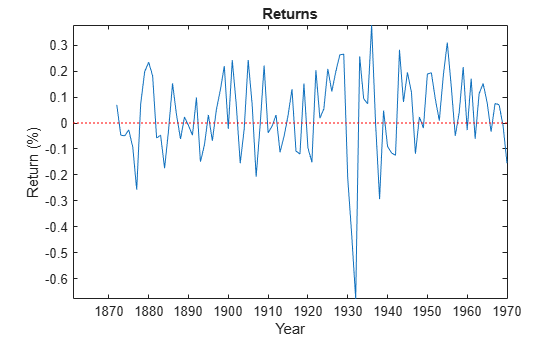
The return series does not seem to have a conditional mean offset, and seems to exhibit volatility clustering. That is, the variability is smaller for earlier years than it is for later years. For this example, assume that an GJR(1,1) model is appropriate for this series.

Create a GJR(1,1) model. The conditional mean offset is zero by default. The software includes a conditional variance model constant by default.

Mdl = gjr('GARCHLags',1,'ARCHLags',1,'LeverageLags',1);

Fit the GJR(1,1) model to the data.

EstMdl = estimate(Mdl,sp);

 
    GJR(1,1) Conditional Variance Model (Gaussian Distribution):
 
                     Value      StandardError    TStatistic     PValue 
                   _________    _____________    __________    ________

    Constant       0.0045728      0.0044199        1.0346       0.30086
    GARCH{1}         0.55808           0.24        2.3253      0.020057
    ARCH{1}          0.20461        0.17886         1.144       0.25263
    Leverage{1}      0.18066        0.26802       0.67406       0.50027

EstMdl is a fully specified gjr model object. That is, it does not contain NaN values. You can assess the adequacy of the model by generating residuals using infer, and then analyzing them.

To simulate conditional variances or responses, pass EstMdl to simulate.

To forecast innovations, pass EstMdl to forecast.

Simulate GJR Model Observations and Conditional Variances

Simulate conditional variance or response paths from a fully specified gjr model object. That is, simulate from an estimated gjr model or a known gjr model in which you specify all parameter values.

Load the Nelson-Plosser data set. Convert the yearly stock price indices to returns.

load Data_NelsonPlosser;
sp = price2ret(DataTable.SP);

Create a GJR(1,1) model. Fit the model to the return series.

Mdl = gjr(1,1);
EstMdl = estimate(Mdl,sp);

 
    GJR(1,1) Conditional Variance Model (Gaussian Distribution):
 
                     Value      StandardError    TStatistic     PValue 
                   _________    _____________    __________    ________

    Constant       0.0045728      0.0044199        1.0346       0.30086
    GARCH{1}         0.55808           0.24        2.3253      0.020057
    ARCH{1}          0.20461        0.17886         1.144       0.25263
    Leverage{1}      0.18066        0.26802       0.67406       0.50027

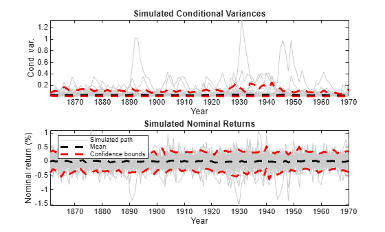
Simulate 100 paths of conditional variances and responses from the estimated GJR model.

numObs = numel(sp); % Sample size (T)
numPaths = 100;     % Number of paths to simulate
rng(1);             % For reproducibility
[VSim,YSim] = simulate(EstMdl,numObs,'NumPaths',numPaths);

VSim and YSim are T-by- numPaths matrices. Rows correspond to a sample period, and columns correspond to a simulated path.

Plot the average and the 97.5% and 2.5% percentiles of the simulated paths. Compare the simulation statistics to the original data.

dates = dates(2:end);
VSimBar = mean(VSim,2);
VSimCI = quantile(VSim,[0.025 0.975],2);
YSimBar = mean(YSim,2);
YSimCI = quantile(YSim,[0.025 0.975],2);

figure;
subplot(2,1,1);
h1 = plot(dates,VSim,'Color',0.8*ones(1,3));
hold on;
h2 = plot(dates,VSimBar,'k--','LineWidth',2);
h3 = plot(dates,VSimCI,'r--','LineWidth',2);
hold off;
title('Simulated Conditional Variances');
ylabel('Cond. var.');
xlabel('Year');
axis tight;

subplot(2,1,2);
h1 = plot(dates,YSim,'Color',0.8*ones(1,3));
hold on;
h2 = plot(dates,YSimBar,'k--','LineWidth',2);
h3 = plot(dates,YSimCI,'r--','LineWidth',2);
hold off;
title('Simulated Nominal Returns');
ylabel('Nominal return (%)');
xlabel('Year');
axis tight;
legend([h1(1) h2 h3(1)],{'Simulated path' 'Mean' 'Confidence bounds'},...
    'FontSize',7,'Location','NorthWest');

Forecast GJR Model Conditional Variances

Forecast conditional variances from a fully specified gjr model object. That is, forecast from an estimated gjr model or a known gjr model in which you specify all parameter values.

Load the Nelson-Plosser data set. Convert the yearly stock price indices (SP) to returns.

load Data_NelsonPlosser;
sp = price2ret(DataTable.SP);

Create a GJR(1,1) model and fit it to the return series.

Mdl = gjr('GARCHLags',1,'ARCHLags',1,'LeverageLags',1);
EstMdl = estimate(Mdl,sp);

 
    GJR(1,1) Conditional Variance Model (Gaussian Distribution):
 
                     Value      StandardError    TStatistic     PValue 
                   _________    _____________    __________    ________

    Constant       0.0045728      0.0044199        1.0346       0.30086
    GARCH{1}         0.55808           0.24        2.3253      0.020057
    ARCH{1}          0.20461        0.17886         1.144       0.25263
    Leverage{1}      0.18066        0.26802       0.67406       0.50027

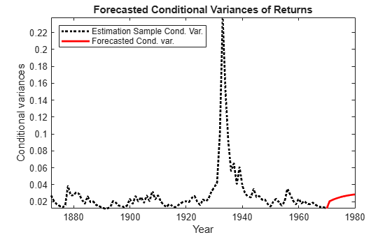
Forecast the conditional variance of the nominal return series 10 years into the future using the estimated GJR model. Specify the entire return series as presample observations. The software infers presample conditional variances using the presample observations and the model.

numPeriods = 10;
vF = forecast(EstMdl,numPeriods,sp);

Plot the forecasted conditional variances of the nominal returns. Compare the forecasts to the observed conditional variances.

v = infer(EstMdl,sp);
nV = size(v,1);
dates = dates((end - nV + 1):end);

figure;
plot(dates,v,'k:','LineWidth',2);
hold on;
plot(dates(end):dates(end) + 10,[v(end);vF],'r','LineWidth',2);
title('Forecasted Conditional Variances of Returns');
ylabel('Conditional variances');
xlabel('Year');
axis tight;
legend({'Estimation Sample Cond. Var.','Forecasted Cond. var.'},...
    'Location','NorthWest');

More About

GJR Model

The Glosten, Jagannathan, and Runkle (GJR) model is a dynamic model that addresses conditional heteroscedasticity, or volatility clustering, in an innovations process. Volatility clustering occurs when an innovations process does not exhibit significant autocorrelation, but the variance of the process changes with time.

The GJR model is a generalization of the GARCH model that is appropriate for modeling asymmetric volatility clustering [1]. Specifically, the model posits that the current conditional variance is the sum of these linear processes, with coefficients:

• Past conditional variances (the GARCH component or polynomial).

• Past squared innovations (the ARCH component or polynomial).

• Past squared, negative innovations (the leverage component or polynomial).

Consider the time series

$$y_t=\mu +{\epsilon }_t,$$

where $${\epsilon }_t={\sigma }_t{z}_t.$$ The GJR(P,Q) conditional variance process, $${\sigma }_t^2$$, has the form

$${\sigma }_t^2=\kappa +{\displaystyle \sum _{i=1}^P{\gamma }_i{\sigma }_{t-i}^2}+{\displaystyle \sum _{j=1}^Q{\alpha }_j}{\epsilon }_{t-j}^2+{\displaystyle \sum _{j=1}^Q{\xi }_j}I\left[{\epsilon }_{t-j}<0\right]{\epsilon }_{t-j}^2.$$

The table shows how the variables correspond to the properties of the gjr object. In the table, I[x < 0] = 1, and 0 otherwise.

Variable	Description	Property
μ	Innovation mean model constant offset	'Offset'
κ > 0	Conditional variance model constant	'Constant'
γj	GARCH component coefficients	'GARCH'
αj	ARCH component coefficients	'ARCH'
ξj	Leverage component coefficients	'Leverage'
zt	Series of independent random variables with mean 0 and variance 1	'Distribution'

For stationarity and positivity, GJR models use these constraints:

• $$\kappa >0$$

• $${\gamma }_i\ge 0,{\alpha }_j\ge 0$$

• $${\alpha }_j+{\xi }_j\ge 0$$

• $${\displaystyle {\sum }_{i=1}^P{\gamma }_i}+{\displaystyle {\sum }_{j=1}^Q{\alpha }_j+\frac{1}{2}}{\displaystyle {\sum }_{j=1}^Q{\xi }_j}<1$$

GJR models are appropriate when negative shocks of contribute more to volatility than positive shocks [2].

If all leverage coefficients are zero, then the GJR model reduces to the GARCH model. Because the GARCH model is nested in the GJR model, you can use likelihood ratio tests to compare a GARCH model fit against a GJR model fit.

Tips

You can specify a gjr model as part of a composition of conditional mean and variance models. For details, see arima.

References

[1] Glosten, L. R., R. Jagannathan, and D. E. Runkle. “On the Relation between the Expected Value and the Volatility of the Nominal Excess Return on Stocks.” The Journal of Finance. Vol. 48, No. 5, 1993, pp. 1779–1801.

[2] Tsay, R. S. Analysis of Financial Time Series. 3rd ed. Hoboken, NJ: John Wiley & Sons, Inc., 2010.

Version History

Introduced in R2012a

R2023a: Name a GJR model response series

Name the response series of a GJR model by setting the SeriesName property of the associated model to a string scalar. When you supply input response data to model object functions in a table or timetable, the functions choose the variable with name SeriesName as the response variable by default.

R2018a: Describe a GJR model

Describe a GJR model by setting the Description property to a string scalar.

R2018a: Use indices that are consistent with MATLAB cell array indexing

The indices of cell arrays of lag operator polynomial coefficients follow MATLAB cell array indexing rules.

Affected model properties are GARCH, ARCH, and Leverage properties.

Update code

• You cannot access any lag-zero coefficients by using an index of 0. For example, Mdl.AR{0} issues an error.

  Remove any instances of such indices of zero from your code. The value of all lag-zero coefficients is 1 except for the lag operator polynomial corresponding to the ARCH property, which has the value 0.

• You cannot index beyond the maximal lag in the polynomial. For example, if Mdl.P is 4, then Mdl.ARCH{p} issues an error when p is greater than 4. For details on the maximal lags of the lag operator polynomials, see the corresponding property descriptions.

  Remove any instances of such indices beyond the maximal lag from your code. All coefficients beyond the maximal lag are 0.

Models store innovation distribution name as a string scalar

The Name field of the Distribution property of gjr model objects stores the innovation distribution name as a string scalar, for example, "Gaussian" for Gaussian innovations.

Before R2018a, MATLAB stored the innovation distribution name as a character vector, for example 'Gaussian' for Gaussian innovations. Although most text-data operations accept character vectors and string scalars for text-data input, there are some differences between the two data types. For more details, see Text in String and Character Arrays.