polyest

Estimate polynomial model using time- or frequency-domain data

Syntax

sys = polyest(tt,[na nb nc nd nf nk])
sys = polyest(u,y,[na nb nc nd nf nk])
sys = polyest(data,[na nb nc nd nf nk])
sys = polyest(___,Name,Value)
sys = polyest(tt,init_sys)
sys = polyest(u,y,init_sys)
sys = polyest(tt,init_sys)
sys = polyest(___, opt)
[sys,ic] = polyest(___)


Description

sys = polyest(tt,[na nb nc nd nf nk]) estimates a polynomial model sys using the data contained in the variables of timetable tt. The software uses the first Nu variables as inputs and the next Ny variables as outputs, where Nu and Ny are determined from the dimensions of the specified polynomial orders.

sys is of the form

$$A(q)y(t)=\frac{B(q)}{F(q)}u(t-nk)+\frac{C(q)}{D(q)}e(t)$$

A(q), B(q), F(q), C(q) and D(q) are polynomial matrices. u(t) is the input, and nk is the input delay. y(t) is the output and e(t) is the disturbance signal. na ,nb, nc, nd and nf are the orders of the A(q), B(q), C(q), D(q) and F(q) polynomials, respectively.

To select specific input and output channels from tt, use name-value syntax to set 'InputName' and 'OutputName' to the corresponding timetable variable names.

sys = polyest(u,y,[na nb nc nd nf nk]) uses the time-domain input and output signals in the comma-separated matrices u,y. The software assumes that the data sample time is 1 second. To change the sample time, set Ts using name-value syntax.

sys = polyest(data,[na nb nc nd nf nk]) uses the time-domain or frequency-domain data in the data object data.

sys = polyest(___,Name,Value) estimates a polynomial model with additional attributes of the estimated model structure specified by one or more Name,Value arguments. You can use this syntax with any of the previous input-argument combinations.

sys = polyest(tt,init_sys) estimates a polynomial model using the linear system init_sys to configure the initial parameterization for estimation using the timetable tt.

sys = polyest(u,y,init_sys) uses the matrix data u,y for estimation..

sys = polyest(tt,init_sys) uses the data object data, for estimation.

sys = polyest(___, opt) estimates a polynomial model using the option set, opt, to specify estimation behavior.

[sys,ic] = polyest(___) returns the estimated initial conditions as an initialCondition object. Use this syntax if you plan to simulate or predict the model response using the same estimation input data and then compare the response with the same estimation output data. Incorporating the initial conditions yields a better match during the first part of the simulation.

Input Arguments

tt	Estimation data, specified as a timetable that uses a regularly spaced time vector. tt contains variables representing input and output channels. For multiexperiment data, tt is a cell array of timetables of length Ne, where Ne is the number of experiments The software determines the number of input and output channels to use for estimation from the dimensions of the specified polynomial orders. The input/output channel selection depends on whether the 'InputName' and 'OutputName' name-value arguments are specified. If 'InputName' and 'OutputName' are not specified, then the software uses the first Nu variables of tt as inputs and the next Ny variables of tt as outputs. If 'InputName' and 'OutputName' are specified, then the software uses the specified variables. The number of specified input and output names must be consistent with Nu and Ny. For functions that can estimate a time series model, where there are no inputs, 'InputName' does not need to be specified. For more information about working with estimation data types, see Data Domains and Data Types in System Identification Toolbox.
u, y	Estimation data, specified for SISO systems as a comma-separated pair of Ns-by-1 real-valued matrices that contain uniformly sampled input and output time-domain signal values. Here, Ns is the number of samples. For MIMO systems, specify u,y as an input/output matrix pair with the following dimensions: u — Ns-by-Nu, where Nu is the number of inputs. y — Ns-by-Ny, where Ny is the number of outputs. For multiexperiment data, specify u,y as a pair of 1-by-Ne cell arrays, where Ne is the number of experiments. The sample times of all the experiments must match. For time series data, which contains only outputs and no inputs, specify y only. For more information about working with estimation data types, see Data Domains and Data Types in System Identification Toolbox.
data	Estimation data. For time-domain estimation, data is an iddata object containing the input and output signal values. You can estimate only discrete-time models using time-domain data. For estimating continuous-time models using time-domain data, see tfest. For frequency-domain estimation, data can be one of the following: Recorded frequency response data (frd (Control System Toolbox) or idfrd) iddata object with its properties specified as follows: InputData — Fourier transform of the input signal OutputData — Fourier transform of the output signal Domain — ‘Frequency’ It may be more convenient to use oe or tfest to estimate a model for frequency-domain data.
na	Order of the polynomial A(q). na is an Ny-by-Ny matrix of nonnegative integers. Ny is the number of outputs, and Nu is the number of inputs. na must be zero if you are estimating a model using frequency-domain data.
nb	Order of the polynomial B(q) + 1. nb is an Ny-by-Nu matrix of nonnegative integers. Ny is the number of outputs, and Nu is the number of inputs.
nc	Order of the polynomial C(q). nc is a column vector of nonnegative integers of length Ny. Ny is the number of outputs. nc must be zero if you are estimating a model using frequency-domain data.
nd	Order of the polynomial D(q). nd is a column vector of nonnegative integers of length Ny. Ny is the number of outputs. nd must be zero if you are estimating a model using frequency-domain data.
nf	Order of the polynomial F(q). nf is an Ny-by-Nu matrix of nonnegative integers. Ny is the number of outputs, and Nu is the number of inputs.
nk	Input delay in number of samples, expressed as fixed leading zeros of the B polynomial. nk is an Ny-by-Nu matrix of nonnegative integers. nk must be zero when estimating a continuous-time model.
opt	Estimation options. opt is an options set, created using polyestOptions, that specifies estimation options including: Estimation objective Handling of initial conditions Numerical search method to be used in estimation
init_sys	Linear system that configures the initial parameterization of sys. You obtain init_sys by either performing an estimation using measured data or by direct construction. If init_sys is an idpoly model, polyest uses the parameters and constraints defined in init_sys as the initial guess for estimating sys. Use the Structure property of init_sys to configure initial guesses and constraints for A(q), B(q), F(q), C(q), and D(q). For example: To specify an initial guess for the A(q) term of init_sys, set init_sys.Structure.A.Value as the initial guess. To specify constraints for the B(q) term of init_sys: Set init_sys.Structure.B.Minimum to the minimum B(q) coefficient values. Set init_sys.Structure.B.Maximum to the maximum B(q) coefficient values. Set init_sys.Structure.B.Free to indicate which B(q) coefficients are free for estimation. If init_sys is not an idpoly model, the software first converts init_sys to a polynomial model. polyest uses the parameters of the resulting model as the initial guess for estimation. If opt is not specified, and init_sys is created by estimation, then the estimation options from init_sys.Report.OptionsUsed are used.

Name-Value Arguments

Specify optional pairs of arguments as Name1=Value1,...,NameN=ValueN, where Name is the argument name and Value is the corresponding value. Name-value arguments must appear after other arguments, but the order of the pairs does not matter.

Before R2021a, use commas to separate each name and value, and enclose Name in quotes.

InputName	Input channel names for timetable data, specified as a string, a character vector, or an array or cell array of strings or character vectors. By default, the software interprets all but the last variable in tt as input channels. When you want to select a subset of the timetable variables as input channels use 'InputName' to identify them. For example, sys = polyest(tt,__,'InputName',["u1" "u2"]) selects the variables u1 and u2 as the input channels for the estimation.
OutputName	Output channel names for timetable data, specified as a string, a character vector, or an array or cell array of strings or character vectors. By default, the software interprets the last variable in tt as the sole output channel. When you want to select a subset of the timetable variables as output channels, use 'OutputName' to identify them. For example, sys = polyest(tt,__,'OutputName',["y1" "y3"]) selects the variables y1 and y3 as the output channels for the estimation.
Ts	Sample time, specified as the comma-separated pair consisting of 'Ts' and the sample time in seconds. When you use matrix-based data (u,y), you must specify 'Ts' if you require a sample time other than the assumed sample time of 1 second. To obtain the data sample time for a timetable tt, use the timetable property tt.Properties.Timestep. Example: polyest(umat1,ymat1,___,'Ts',0.08) computes a model with sample time of 0.08 seconds.
IODelay	Transport delays. IODelay is a numeric array specifying a separate transport delay for each input/output pair. For continuous-time systems, specify transport delays in the time unit stored in the TimeUnit property. For discrete-time systems, specify transport delays in integer multiples of the sample time, Ts. For a MIMO system with Ny outputs and Nu inputs, set IODelay to a Ny-by-Nu array. Each entry of this array is a numerical value that represents the transport delay for the corresponding input/output pair. You can also set IODelay to a scalar value to apply the same delay to all input/output pairs. Default: 0 for all input/output pairs
InputDelay	Input delay for each input channel, specified as a scalar value or numeric vector. For continuous-time systems, specify input delays in the time unit stored in the TimeUnit property. For discrete-time systems, specify input delays in integer multiples of the sample time Ts. For example, InputDelay = 3 means a delay of three sample times. For a system with Nu inputs, set InputDelay to an Nu-by-1 vector. Each entry of this vector is a numerical value that represents the input delay for the corresponding input channel. You can also set InputDelay to a scalar value to apply the same delay to all channels. Default: 0
IntegrateNoise	Logical vector specifying integrators in the noise channel. IntegrateNoise is a logical vector of length Ny, where Ny is the number of outputs. Setting IntegrateNoise to true for a particular output results in the model: $$A(q)y(t)=\frac{B(q)}{F(q)}u(t-nk)+\frac{C(q)}{D(q)}\frac{e(t)}{1-q^{-1}}$$ Where, $$\frac{1}{1-q^{-1}}$$ is the integrator in the noise channel, e(t). Use IntegrateNoise to create an ARIMAX model. For example, load iddata1 z1; z1 = iddata(cumsum(z1.y),cumsum(z1.u),z1.Ts,'InterSample','foh'); sys = polyest(z1, [2 2 2 0 0 1],'IntegrateNoise',true);

Output Arguments

sys

Polynomial model, returned as an idpoly model. This model is created using the specified model orders, delays, and estimation options. If data.Ts is zero, sys is a continuous-time model representing: $$Y(s)=\frac{B(s)}{F(s)}U(s)+E(s)$$ Y(s), U(s) and E(s) are the Laplace transforms of the time-domain signals y(t), u(t) and e(t), respectively. Information about the estimation results and options used is stored in the Report property of the model. Report have the following fields: Report Field Description Status Summary of the model status, which indicates whether the model was created by construction or obtained by estimation. Method Estimation command used. InitialCondition Handling of initial conditions during model estimation, returned as one of the following values: 'zero' — The initial conditions were set to zero. 'estimate' — The initial conditions were treated as independent estimation parameters. 'backcast' — The initial conditions were estimated using the best least squares fit. This field is especially useful to view how the initial conditions were handled when the InitialCondition option in the estimation option set is 'auto'. Fit Quantitative assessment of the estimation, returned as a structure. See Loss Function and Model Quality Metrics for more information on these quality metrics. The structure has the following fields: Field Description FitPercent Normalized root mean squared error (NRMSE) measure of how well the response of the model fits the estimation data, expressed as the percentage fitpercent = 100(1-NRMSE). LossFcn Value of the loss function when the estimation completes. MSE Mean squared error (MSE) measure of how well the response of the model fits the estimation data. FPE Final prediction error for the model. AIC Raw Akaike Information Criteria (AIC) measure of model quality. AICc Small-sample-size corrected AIC. nAIC Normalized AIC. BIC Bayesian Information Criteria (BIC). Parameters Estimated values of model parameters. OptionsUsed Option set used for estimation. If no custom options were configured, this is a set of default options. See polyestOptions for more information. RandState State of the random number stream at the start of estimation. Empty, [], if randomization was not used during estimation. For more information, see rng. DataUsed Attributes of the data used for estimation, returned as a structure with the following fields. Field Description Name Name of the data set. Type Data type. Length Number of data samples. Ts Sample time. InterSample Input intersample behavior, returned as one of the following values: 'zoh' — Zero-order hold maintains a piecewise-constant input signal between samples. 'foh' — First-order hold maintains a piecewise-linear input signal between samples. 'bl' — Band-limited behavior specifies that the continuous-time input signal has zero power above the Nyquist frequency. InputOffset Offset removed from time-domain input data during estimation. For nonlinear models, it is []. OutputOffset Offset removed from time-domain output data during estimation. For nonlinear models, it is []. Termination Termination conditions for the iterative search used for prediction error minimization, returned as a structure with the following fields: Field Description WhyStop Reason for terminating the numerical search. Iterations Number of search iterations performed by the estimation algorithm. FirstOrderOptimality $$\infty$$-norm of the gradient search vector when the search algorithm terminates. FcnCount Number of times the objective function was called. UpdateNorm Norm of the gradient search vector in the last iteration. Omitted when the search method is 'lsqnonlin' or 'fmincon'. LastImprovement Criterion improvement in the last iteration, expressed as a percentage. Omitted when the search method is 'lsqnonlin' or 'fmincon'. Algorithm Algorithm used by 'lsqnonlin' or 'fmincon' search method. Omitted when other search methods are used. For estimation methods that do not require numerical search optimization, the Termination field is omitted. For more information on using Report, see Estimation Report.

ic

Estimated initial conditions, returned as an initialCondition object or an object array of initialCondition values. For a single-experiment data set, ic represents, in state-space form, the free response of the transfer function model (A and C matrices) to the estimated initial states (x0). For a multiple-experiment data set with Ne experiments, ic is an object array of length Ne that contains one set of initialCondition values for each experiment. If polyest returns ic values of 0 and the you know that you have non-zero initial conditions, set the 'InitialCondition' option in polyestOptions to 'estimate' and pass the updated option set to polyest. For example: opt = polyestOptions('InitialCondition','estimate') [sys,ic] = polyest(data,[nb nc nd nf nk],opt) The default 'auto' setting of 'InitialCondition' uses the 'zero' method when the initial conditions have a negligible effect on the overall estimation-error minimization process. Specifying 'estimate' ensures that the software estimates values for ic. For more information, see initialCondition. For an example of using this argument, see Obtain Initial Conditions.

Examples

Estimate Polynomial Model with Redundant Parameterization

Estimate a model with redundant parameterization. That is, a model with all polynomials ($$A$$, $$B$$, $$C$$, $$D$$, and $$F$$) active.

Load estimation data.

load sdata2 tt2;

Specify the model orders and delays.

na = 2; 
nb = 2; 
nc = 3; 
nd = 3; 
nf = 2; 
nk = 1;

Estimate the model.

sys = polyest(tt2,[na nb nc nd nf nk]);

Compare the model output to the measured output.

compare(tt2,sys)

Estimate Polynomial Model Using Regularization

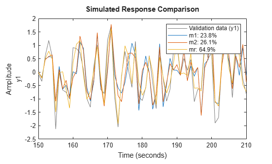
Estimate a regularized polynomial model by converting a regularized ARX model.

Load estimation data.

load regularizationExampleData.mat m0simdata;

Estimate an unregularized polynomial model of order 20.

m1 = polyest(m0simdata(1:150),[0 20 20 20 20 1]);

Estimate a regularized polynomial model of the same order. Determine the Lambda value by trial and error.

opt = polyestOptions;
opt.Regularization.Lambda = 1;
m2 = polyest(m0simdata(1:150),[0 20 20 20 20 1],opt);

Obtain a lower-order polynomial model by converting a regularized ARX model and reducing its order. Use arxregul to determine the regularization parameters.

[L,R] = arxRegul(m0simdata(1:150),[30 30 1]);
opt1 = arxOptions;
opt1.Regularization.Lambda = L;
opt1.Regularization.R = R;
m0 = arx(m0simdata(1:150),[30 30 1],opt1);
mr = idpoly(balred(idss(m0),7));

Compare the model outputs against the data.

opt2 = compareOptions('InitialCondition','z');
compare(m0simdata(150:end),m1,m2,mr,opt2);

Estimate ARIMAX model

Load input/output data and create cumulative sum input and output signals for estimation.

load iddata1 z1
data = iddata(cumsum(z1.y),cumsum(z1.u),z1.Ts,'InterSample','foh');

Specify the model polynomial orders. Set the orders of the inactive polynomials, $$D$$ and $$F$$, to 0.

na = 2; 
nb = 2; 
nc = 2; 
nd = 0; 
nf = 0; 
nk = 1;

Identify an ARIMAX model by setting the 'IntegrateNoise' option to true.

sys = polyest(data,[na nb nc nd nf nk],'IntegrateNoise',true);

Compare the simulated model output to the measured output.

compare(data,sys)

Estimate Multi-Output ARMAX Model

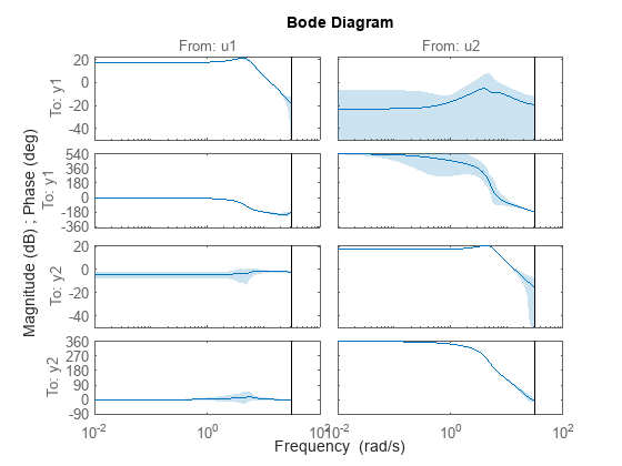
Estimate a multi-output ARMAX model for a multi-input, multi-output data set.

Load estimation data.

load iddata1 z1
load iddata2 z2
data = [z1 z2(1:300)];

data is a data set with 2 inputs and 2 outputs. The first input affects only the first output. Similarly, the second input affects only the second output.

Specify the model orders and delays. The F and D polynomials are inactive.

na = [2 2; 2 2]; 
nb = [2 2; 3 4]; 
nk = [1 1; 0 0]; 
nc = [2;2]; 
nd = [0;0]; 
nf = [0 0; 0 0];

Estimate the model.

sys = polyest(data,[na nb nc nd nf nk]);

In the estimated ARMAX model, the cross terms, which model the effect of the first input on the second output and vice versa, are negligible. If you assigned higher orders to those dynamics, their estimation would show a high level of uncertainty.

Analyze the results.

h = bodeplot(sys);
showConfidence(h,3)

The responses from the cross terms show larger uncertainty.

Obtain Initial Conditions

Load the data.

load iddata1ic z1i

Estimate a polynomial model sys and return the initial conditions in ic.

na = 2;
nb = 2;
nc = 3;
nd = 3;
nf = 2;
nk = 1;
[sys,ic] = polyest(z1i,[na nb nc nd nf nk]);
ic

ic = 
  initialCondition with properties:

     A: [7x7 double]
    X0: [7x1 double]
     C: [0 0 0 0 0 0 1]
    Ts: 0.1000

ic is an initialCondition object that encapsulates the free response of sys, in state-space form, to the initial state vector in X0. You can incorporate ic when you simulate sys with the z1i input signal and compare the response with the z1i output signal.

Tips

• In most situations, all the polynomials of an identified polynomial model are not simultaneously active. Set one or more of the orders na, nc, nd and nf to zero to simplify the model structure.

  For example, you can estimate an Output-Error (OE) model by specifying na, nc and nd as zero.

  Alternatively, you can use a dedicated estimating function for the simplified model structure. Linear polynomial estimation functions include oe, bj, arx and armax.

Alternatives

• To estimate a polynomial model using time-series data, use ar.

• Use polyest to estimate a polynomial of arbitrary structure. If the structure of the estimated polynomial model is known, that is, you know which polynomials will be active, then use the appropriate dedicated estimating function. For examples, for an ARX model, use arx. Other polynomial model estimating functions include, oe, armax, and bj.

• To estimate a continuous-time transfer function, use tfest. You can also use oe, but only with continuous-time frequency-domain data.

Version History

Introduced in R2012a

R2022b: Time-domain estimation data is accepted in the form of timetables and matrices

Most estimation, validation, analysis, and utility functions now accept time-domain input/output data in the form of a single timetable that contains both input and output data or a pair of matrices that contain the input and output data separately. These functions continue to accept iddata objects as a data source as well, for both time-domain and frequency-domain data.

R2018a: Advanced Options are deprecated for SearchOptions when SearchMethod is 'lsqnonlin'

Specification of lsqnonlin- related advanced options are deprecated, including the option to invoke parallel processing when estimating using the lsqnonlin search method, or solver, in Optimization Toolbox™.