Estimate Model Using Zero/Pole/Gain Parameters
This example shows how to estimate a model that is parameterized by poles, zeros, and gains. The example requires Control System Toolbox™ software.
You parameterize the model using complex-conjugate pole/zero pairs. When you parameterize a real, grey-box model using complex-conjugate pairs of parameters, the software updates parameter values such that the estimated values are also complex conjugate pairs.
Load the measured data.
load zpkestdata zd;
The variable zd, which contains measured data, is loaded into the MATLAB® workspace.
plot(zd);
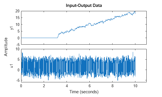
The output shows an input delay of approximately 3.14 seconds.
Estimate the model using the zero-pole-gain (zpk) form using the zpkestODE function. To view this function, enter
type zpkestODEfunction [a,b,c,d] = zpkestODE(z,p,k,Ts,varargin) %zpkestODE ODE file that parameterizes a state-space model using poles and %zeros as its parameters. % % Requires Control System Toolbox. % Copyright 2011 The MathWorks, Inc. sysc = zpk(z,p,k); if Ts==0 [a,b,c,d] = ssdata(sysc); else [a,b,c,d] = ssdata(c2d(sysc,Ts,'foh')); end
Create a linear grey-box model associated with the ODE function.
Assume that the model has five poles and four zeros. Assume that two of the poles and two of the zeros are complex conjugate pairs.
z = [-0.5+1i, -0.5-1i, -0.5, -1];
p = [-1.11+2i, -1.11-2i, -3.01, -4.01, -0.02];
k = 10.1;
parameters = {z,p,k};
Ts = 0;
odefun = @zpkestODE;
init_sys = idgrey(odefun,parameters,'cd',{},Ts,'InputDelay',3.14);z, p, and k are the initial guesses for the model parameters.
init_sys is an idgrey model that is associated with the zpkestODE.m function. The 'cd' flag indicates that the ODE function, zpkestODE, returns continuous or discrete models, depending on the sampling period.
Evaluate the quality of the fit provided by the initial model.
compareOpt = compareOptions('InitialCondition','zero');
compare(zd,init_sys,compareOpt);
legend(Interpreter="none")
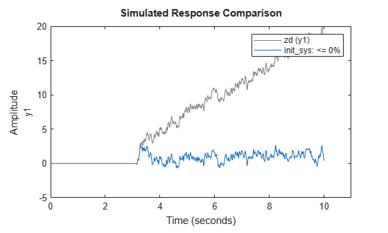
The initial model provides a poor fit.
Specify estimation options.
opt = greyestOptions('InitialState','zero','DisturbanceModel','none','SearchMethod','gna');
Estimate the model.
sys = greyest(zd,init_sys,opt);
sys, an idgrey model, contains the estimated zero-pole-gain model parameters.
Compare the estimated and initial parameter values.
[getpvec(init_sys) getpvec(sys)]
ans = 10×2 complex

  -0.5000 + 1.0000i  -1.6158 + 1.6173i
  -0.5000 - 1.0000i  -1.6158 - 1.6173i
  -0.5000 + 0.0000i  -0.9417 + 0.0000i
  -1.0000 + 0.0000i  -1.4099 + 0.0000i
  -1.1100 + 2.0000i  -2.4050 + 1.4340i
  -1.1100 - 2.0000i  -2.4050 - 1.4340i
  -3.0100 + 0.0000i  -2.3387 + 0.0000i
  -4.0100 + 0.0000i  -2.3392 + 0.0000i
  -0.0200 + 0.0000i  -0.0082 + 0.0000i
  10.1000 + 0.0000i   9.7881 + 0.0000i
The getpvec command returns the parameter values for a model. In the output above, each row displays corresponding initial and estimated parameter values. All parameters that were initially specified as complex conjugate pairs remain so after estimation.
Evaluate the quality of the fit provided by the estimated model.
compare(zd,init_sys,sys,compareOpt);
legend(Interpreter="none")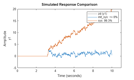
sys provides a closer fit (98.35%) to the measured data.
See Also
idgrey | greyest | getpvec | ssdata | c2d