Estimate Coefficients of ODEs to Fit Given Solution
This example shows how to estimate model parameters using linear and nonlinear grey-box modeling.
Use grey-box identification to estimate coefficients of ODEs that describe the model dynamics to fit a given response trajectory.
For linear dynamics, represent the model using a linear grey-box model (
idgrey). Estimate the model coefficients usinggreyest.For nonlinear dynamics, represent the model using a nonlinear grey-box model (
idnlgrey). Estimate the model coefficients usingnlgreyest.
In this example, you estimate the value of the friction coefficient of a simple pendulum using its oscillation data. The equation of motion of a simple pendulum is:
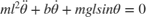
 is the angular displacement of the pendulum relative to its state of rest.
 g is the gravitational acceleration constant. m is the mass of the pendulum and l is the length of the pendulum. b is the viscous friction coefficient whose value is estimated to fit the given angular displacement data. There is no external driving force that is contributing to the pendulum motion.
Load Measured Data
load pendulumdata
data = iddata(y,[],0.1,'Name','Pendulum');
data.OutputName = 'Pendulum position';
data.OutputUnit = 'rad';
data.Tstart = 0;
data.TimeUnit = 's';
The measured angular displacement data is loaded and saved as data, an iddata object with a sample time of 0.1 seconds. The set command is used to specify data attributes such as the output name, output unit, and the start time and units of the time vector.
Perform Linear Grey-Box Estimation
Assuming that the pendulum undergoes only small angular displacements, the equation describing the pendulum motion can be simplified:
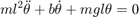
Using the angular displacement ( ) and the angular velocity (
 ) as state variables, the simplified equation can be rewritten in the form:
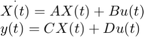
Here,
![$$\begin{array}{l} X(t) = \left[ {\begin{array}{*{20}{c}} \theta \\ {\dot \theta } \end{array}} \right]\\ A = \left[ {\begin{array}{*{20}{c}} 0&1\\ {\frac{{ - g}}{l}}&{\frac{{ - b}}{{m{l^2}}}} \end{array}} \right]\\ B = 0\\ C = \left[ {\begin{array}{*{20}{c}} 1&0 \end{array}} \right]\\ D = 0 \end{array}$$](../../examples/ident/win64/EstimatingCoefficientsOfODEsToFitGivenSolutionExample_eq06570395619421982669.png)
The B and D matrices are zero because there is no external driving force for the simple pendulum.
1. Create an ODE file that relates the model coefficients to its state space representation.
function [A,B,C,D] = LinearPendulum(m,g,l,b,Ts)
A = [0 1; -g/l, -b/m/l^2];
B = zeros(2,0);
C = [1 0];
D = zeros(1,0);
end
The function, LinearPendulum, returns the state space representation of the linear motion model of the simple pendulum using the model coefficients m, g, l, and b. Ts is the sample time. Save this function as LinearPendulum.m. The function LinearPendulum must be on the MATLAB® path. Alternatively, you can specify the full path name for this function.
2. Create a linear grey-box model associated with the LinearPendulum function.
m = 1;
g = 9.81;
l = 1;
b = 0.2;
linear_model = idgrey('LinearPendulum',{m,g,l,b},'c');
m, g and, l specify the values of the known model coefficients. b specifies the initial guess for the viscous friction coefficient. The 'c' input argument in the call to idgrey specifies linear_model as a continuous-time system.
3. Specify m, g, and l as known parameters.
linear_model.Structure.Parameters(1).Free = false;
linear_model.Structure.Parameters(2).Free = false;
linear_model.Structure.Parameters(3).Free = false;
As defined in the previous step, m, g, and l are the first three parameters of linear_model. Using the Structure.Parameters.Free field for each of the parameters, m, g, and l are specified as fixed values.
4. Create an estimation option set that specifies the initial state to be estimated and turns on the estimation progress display. Also force the estimation algorithm to return a stable model. This option is available only for linear model (idgrey) estimation.
opt = greyestOptions('InitialState','estimate','Display','on');
opt.EnforceStability = true;
5. Estimate the viscous friction coefficient.
linear_model = greyest(data,linear_model,opt);
The greyest command updates the parameter of linear_model.
b_est = linear_model.Structure.Parameters(4).Value;
[linear_b_est,dlinear_b_est] = getpvec(linear_model,'free')
linear_b_est =

    0.1178


dlinear_b_est =

    0.0088
getpvec returns, dlinear_b_est, the 1 standard deviation uncertainty associated with b, the free estimation parameter of linear_model.The estimated value of b, the viscous friction coefficient, using linear grey-box estimation is returned in linear_b_est.
6. Compare the response of the linear grey-box model to the measured data.
compare(data,linear_model)
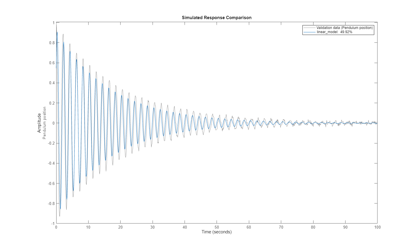
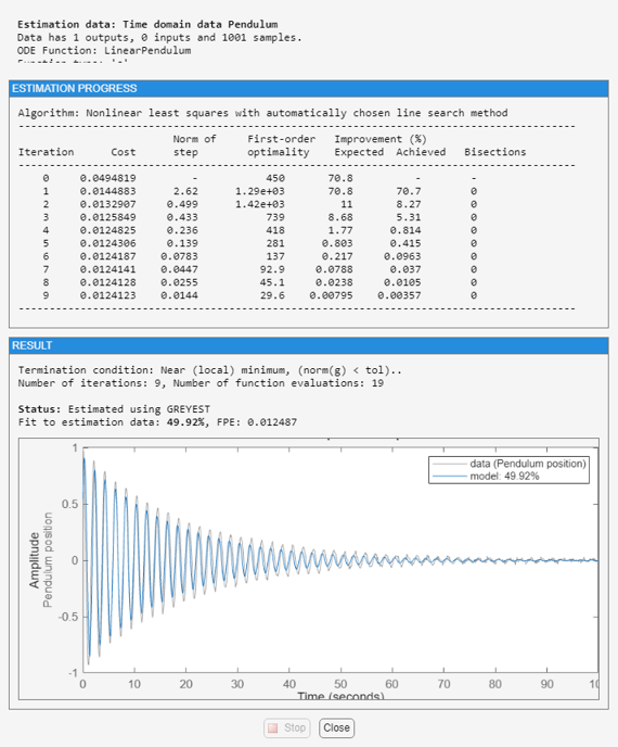
The linear grey-box estimation model provides a 49.9% fit to measured data. The poor fit is due to the assumption that the pendulum undergoes small angular displacements, whereas the measured data shows large oscillations.
Perform Nonlinear Grey-Box Estimation
Nonlinear grey-box estimation requires that you express the differential equation as a set of first order equations.
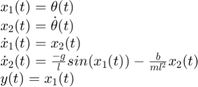
Using the angular displacement () and the angular velocity () as state variables, the equation of motion can be rewritten as a set of first order nonlinear differential equations:
1. Create an ODE file that relates the model coefficients to its nonlinear representation.
function [dx,y] = NonlinearPendulum(t,x,u,m,g,l,b,varargin)

% Output equation.
y = x(1); % Angular position.

% State equations.
dx = [x(2);                             ... % Angular position
      -(g/l)*sin(x(1))-b/(m*l^2)*x(2)   ... % Angular velocity
     ];
end
The function, NonlinearPendulum, returns the state derivatives and output of the nonlinear motion model of the pendulum using the model coefficients m, g, l, and b. Save this function as NonlinearPendulum.m on the MATLAB® path. Alternatively, you can specify the full path name for this function.
2. Create a nonlinear grey-box model associated with the NonlinearPendulum function.
m = 1;
g = 9.81;
l = 1;
b = 0.2;
order         = [1 0 2];
parameters    = {m,g,l,b};
initial_states = [1; 0];
Ts            = 0;
nonlinear_model = idnlgrey('NonlinearPendulum',order,parameters,initial_states,Ts);
3. Specify m, g, and l as known parameters.
setpar(nonlinear_model,'Fixed',{true true true false});
As defined in the previous step, m, g, and l are the first three parameters of nonlinear_model. Using the setpar command, m, g, and l are specified as fixed values and b is specified as a free estimation parameter.
4. Estimate the viscous friction coefficient.
nonlinear_model = nlgreyest(data,nonlinear_model,'Display','Full');
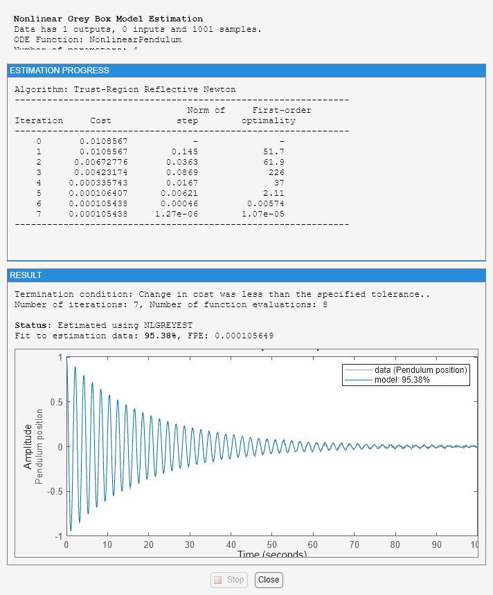
The nlgreyest command updates the parameter of nonlinear_model.
b_est = nonlinear_model.Parameters(4).Value;
[nonlinear_b_est, dnonlinear_b_est] = getpvec(nonlinear_model,'free')
nonlinear_b_est =

    0.1002


dnonlinear_b_est =

    0.0149
getpvec returns, as dnonlinear_b_est, the 1 standard deviation uncertainty associated with b, the free estimation parameter of nonlinear_model.The estimated value of b, the viscous friction coefficient, using nonlinear grey-box estimation is returned in nonlinear_b_est.
5. Compare the response of the linear and nonlinear grey-box models to the measured data.
compare(data,linear_model,nonlinear_model)
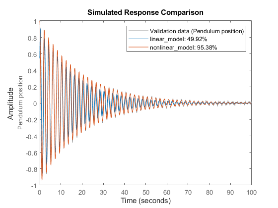
The nonlinear grey-box model estimation provides a closer fit to the measured data.
See Also
idgrey | idnlgrey | greyest | nlgreyest