geoplot
Plot line in geographic coordinates
Syntax
Description
Vector Data
geoplot(
plots a line in geographic coordinates. Specify latitude coordinates in degrees
using lat,lon)lat, and specify longitude coordinates in degrees
using lon. If the current axes is not a geographic or map
axes, or if there is no current axes, then the function plots the line in a new
geographic axes.
Table Data
geoplot(
plots the variables tbl,latvar,lonvar)latvar and lonvar from
the table tbl. To plot one data set, specify one variable for
latvar and one variable for lonvar. To
plot multiple data sets, specify multiple variables for
latvar, lonvar, or both. If both
arguments specify multiple variables, they must specify the same number of
variables. (Since R2022b)
Additional Options
geoplot( displays
the plot in the axes specified by ax,___)ax. Specify the axes as
the first argument in any of the previous syntaxes.
geoplot(___,
specifies properties of the chart line using one or more name-value arguments.
The properties apply to all the plotted lines. For a list of properties, see
Line Properties.Name,Value)
h = geoplot(___)h to modify the properties of the plot after
creating it. For a list of properties, see Line Properties.
Note
Mapping Toolbox™ extends the functionality of the geoplot (MATLAB®) function. It adds support for displaying points, lines, and polygons with coordinates in any supported geographic or projected coordinate reference system (CRS). For the geoplot (Mapping Toolbox) page, see geoplot (Mapping Toolbox).
Examples
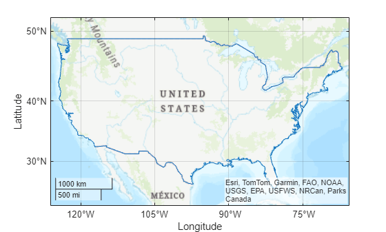
Load a MAT file containing coordinates for the perimeter of the contiguous United States. The variables within the MAT file, uslat and uslon, specify latitude and longitude coordinates, respectively, in degrees. Display the coordinates over a topographic basemap.
load usapolygon.mat
geoplot(uslat,uslon)
geobasemap topographic
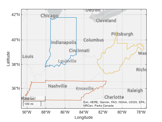
Load a MAT file containing coordinates for each contiguous US state. Extract the coordinates for Indiana, Tennessee, and West Virginia.
load usastates.mat

lat1 = usastates(12).Lat;
lon1 = usastates(12).Lon;

lat2 = usastates(40).Lat;
lon2 = usastates(40).Lon;

lat3 = usastates(46).Lat;
lon3 = usastates(46).Lon;
Display the state outlines using three lines. Zoom out by changing the geographic limits.
geoplot(lat1,lon1,lat2,lon2,lat3,lon3)
geolimits([33.5 42.2],[-93.0 -75.5])
Specify the latitude and longitude coordinates of several points along a highway in Germany. Display the points as a line over the streets basemap using a black dashed line with circle markers.
lat = [48.915 48.907 48.901 48.893 48.887 48.881 48.875 48.869 48.865];
lon = [10.192 10.188 10.182 10.171 10.166 10.165 10.167 10.173 10.184];

geoplot(lat,lon,"k--o")
geobasemap streets

Specify the latitude and longitude coordinates of several points along the Mississippi River.
lat = [32.30 33.92 35.17 36.98 37.69 38.34];
lon = [-91.05 -91.18 -90.09 -89.11 -89.52 -90.37];
Create a line plot from the data. Use the LineSpec option to specify a dashed green line with square markers. Use name-value arguments to specify the line width, marker size, and marker colors.
geoplot(lat,lon,"--gs",LineWidth=2, ...
    MarkerSize=10,MarkerEdgeColor="b", ...
    MarkerFaceColor=[0.5 0.5 0.5])
Zoom out by adjusting the latitude and longitude limits of the plot. Then, change the basemap to a terrain basemap.
geolimits([31.6 38.8],[-97 -83])
geobasemap grayterrain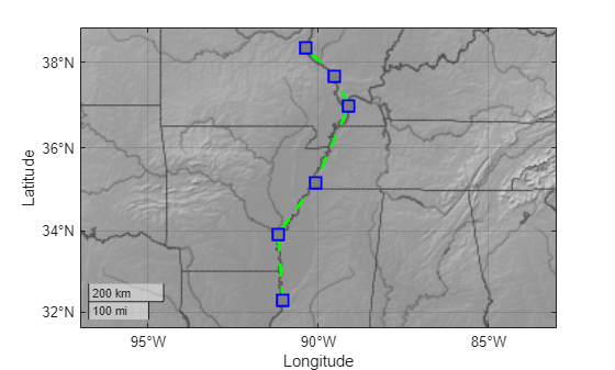
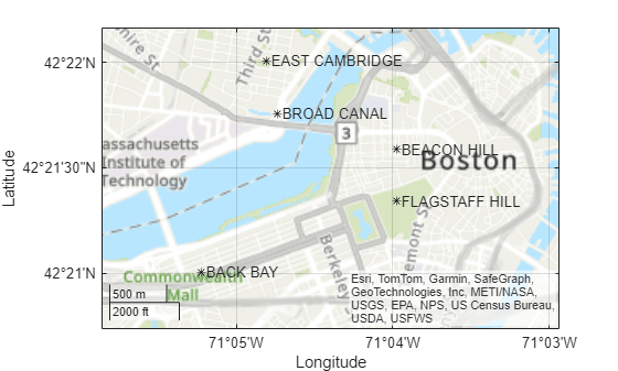
Specify the geographic coordinates and names of several places in Boston.
lat = [42.3501 42.3598 42.3626 42.3668 42.3557];
lon = [-71.0870 -71.0662 -71.0789 -71.0801 -71.0662];
n = [" BACK BAY"," BEACON HILL"," BROAD CANAL"," EAST CAMBRIDGE"," FLAGSTAFF HILL"];
Plot the locations using black star markers over the topographic basemap. Zoom out of the plot by adjusting the limits.
geoplot(lat,lon,"k*")
geobasemap topographic
geolimits([42.3456 42.3694],[-71.0977 -71.0489])
Display the place names at the same locations.
text(lat,lon,n)
Since R2022b
A convenient way to plot data from a table is to pass the table to the geoplot function and specify the variables to plot.
Load a MAT file containing cyclone data [1] into the workspace. Create a table using a subset of the data. The table includes latitude and longitude coordinates in the table variables Latitude and Longitude, respectively.
load cycloneTracks.mat
tbl = cycloneTracks(cycloneTracks.ID == 1320,:);
Plot the latitude and longitude coordinates over a topographic basemap. Return the Line object as h.
h = geoplot(tbl,"Latitude","Longitude");
geobasemap topographic
Change the marker style and color of the plot by setting the Marker and Color properties.
h.Marker = ".";
h.Color = "m";
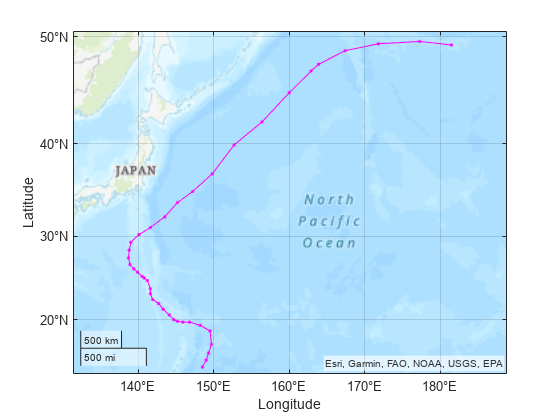
[1] This example uses modified RSMC Best Track Data from the Japan Meteorological Agency.
Input Arguments
Latitude coordinates in degrees, specified as a vector with elements in the range [–90, 90].
Create breaks in the lines using NaN values. For
example, this code plots the first two elements, skips the third element,
and then plots another line using the last two
elements.
geoplot([10 20 NaN 30 40],[10 20 NaN 30 40])
The sizes of lat and lon must
match.
Example: [43.0327 38.8921 44.0435]
Data Types: single | double
Longitude coordinates in degrees, specified as a vector.
Create breaks in the lines using NaN values. For
example, this code plots the first two elements, skips the third element,
and then plots another line using the last two
elements.
geoplot([10 20 NaN 30 40],[10 20 NaN 30 40])
The sizes of lat and lon must
match.
Example: [-107.5556 -77.0269 -72.5565]
Data Types: single | double
Line style, marker, and color, specified as a string scalar or character vector containing symbols. The symbols can appear in any order. You do not need to specify all three characteristics (line style, marker, and color). For example, if you omit the line style and specify the marker, then the plot shows only the marker and no line.
Example: "--or" is a red dashed line with circle markers.
| Line Style | Description | Resulting Line |
|---|---|---|
"-" | Solid line |
|
"--" | Dashed line |
|
":" | Dotted line |
|
"-." | Dash-dotted line |
|
| Marker | Description | Resulting Marker |
|---|---|---|
"o" | Circle |
|
"+" | Plus sign |
|
"*" | Asterisk |
|
"." | Point |
|
"x" | Cross |
|
"_" | Horizontal line |
|
"|" | Vertical line |
|
"square" | Square |
|
"diamond" | Diamond |
|
"^" | Upward-pointing triangle |
|
"v" | Downward-pointing triangle |
|
">" | Right-pointing triangle |
|
"<" | Left-pointing triangle |
|
"pentagram" | Pentagram |
|
"hexagram" | Hexagram |
|
| Color Name | Short Name | RGB Triplet | Appearance |
|---|---|---|---|
"red" | "r" | [1 0 0] |
|
"green" | "g" | [0 1 0] |
|
"blue" | "b" | [0 0 1] |
|
"cyan"
| "c" | [0 1 1] |
|
"magenta" | "m" | [1 0 1] |
|
"yellow" | "y" | [1 1 0] |
|
"black" | "k" | [0 0 0] |
|
"white" | "w" | [1 1 1] |
|
Source table containing the data to plot, specified as a table or timetable.
Table variables containing the latitude coordinates, specified using one of the indexing schemes from the table.
| Indexing Scheme | Examples |
|---|---|
Variable names:
|
|
Variable indices:
|
|
Variable type:
|
|
Regardless of variable names, the axis label on the plot is always
Latitude.
The variables must contain numeric data of type single
or double. The data must be in the range [–90, 90].
If latvar and lonvar both specify
multiple variables, the number of variables must be the same.
Example: geoplot(tbl,["lat1","lat2"],"lon") specifies
the table variables named lat1 and
lat2 for the latitude coordinates.
Example: geoplot(tbl,2,"lon") specifies the second
variable for the latitude coordinates.
Example: geoplot(tbl,vartype("numeric"),"lon") specifies
all numeric variables for the latitude coordinates.
Table variables containing the longitude coordinates, specified using one of the indexing schemes from the table.
| Indexing Scheme | Examples |
|---|---|
Variable names:
|
|
Variable indices:
|
|
Variable type:
|
|
Regardless of variable names, the axis label on the plot is always
Longitude.
The variables you specify must contain numeric data of type
single or double.
If latvar and lonvar both specify
multiple variables, the number of variables must be the same.
Example: geoplot(tbl,"lat",["lon1","lon2"]) specifies
the table variables named lon1 and
lon2 for the longitude coordinates.
Example: geoplot(tbl,"lat",2) specifies the second
variable for the longitude coordinates.
Example: geoplot(tbl,"lat",vartype("numeric")) specifies
all numeric variables for the longitude coordinates.
Target axes, specified as a GeographicAxes
object1
or MapAxes (Mapping Toolbox) object. If you do not specify this argument, then the
geoplot function plots into the current axes,
provided that the current axes is a geographic or map axes object.
Name-Value Arguments
Specify optional pairs of arguments as
Name1=Value1,...,NameN=ValueN, where Name is
the argument name and Value is the corresponding value.
Name-value arguments must appear after other arguments, but the order of the
pairs does not matter.
Example: geoplot(lat,lon,LineWidth=2) plots a line with a line
width of 2 points.
Before R2021a, use commas to separate each name and value, and enclose
Name in quotes.
Example: geoplot(lat,lon,"LineWidth",2) plots a line with a line
width of 2 points.
Note
Use name-value arguments to specify values for the properties of the
Line objects created by this function. The properties
listed here are only a subset. For a full list, see Line Properties.
Property settings apply to all lines in the plot. To set the properties of an
individual line, get a handle to the line by specifying the output argument
h. Then, use dot notation to set properties for an
individual line.
Line color, specified as an RGB triplet, a hexadecimal color code, a color name, or a short name.
For a custom color, specify an RGB triplet or a hexadecimal color code.
An RGB triplet is a three-element row vector whose elements specify the intensities of the red, green, and blue components of the color. The intensities must be in the range
[0,1], for example,[0.4 0.6 0.7].A hexadecimal color code is a string scalar or character vector that starts with a hash symbol (
#) followed by three or six hexadecimal digits, which can range from0toF. The values are not case sensitive. Therefore, the color codes"#FF8800","#ff8800","#F80", and"#f80"are equivalent.
Alternatively, you can specify some common colors by name. This table lists the named color options, the equivalent RGB triplets, and the hexadecimal color codes.
| Color Name | Short Name | RGB Triplet | Hexadecimal Color Code | Appearance |
|---|---|---|---|---|
"red" | "r" | [1 0 0] | "#FF0000" |
|
"green" | "g" | [0 1 0] | "#00FF00" |
|
"blue" | "b" | [0 0 1] | "#0000FF" |
|
"cyan"
| "c" | [0 1 1] | "#00FFFF" |
|
"magenta" | "m" | [1 0 1] | "#FF00FF" |
|
"yellow" | "y" | [1 1 0] | "#FFFF00" |
|
"black" | "k" | [0 0 0] | "#000000" |
|
"white" | "w" | [1 1 1] | "#FFFFFF" |
|
"none" | Not applicable | Not applicable | Not applicable | No color |
This table lists the default color palettes for plots in the light and dark themes.
| Palette | Palette Colors |
|---|---|
Before R2025a: Most plots use these colors by default. |
|
|
|
You can get the RGB triplets and hexadecimal color codes for these palettes using the orderedcolors and rgb2hex functions. For example, get the RGB triplets for the "gem" palette and convert them to hexadecimal color codes.
RGB = orderedcolors("gem");
H = rgb2hex(RGB);
Before R2023b: Get the RGB triplets using RGB =
get(groot,"FactoryAxesColorOrder").
Before R2024a: Get the hexadecimal color codes using H =
compose("#%02X%02X%02X",round(RGB*255)).
Example: "blue"
Example: [0 0 1]
Example: "#0000FF"
Line style, specified as one of the options listed in this table.
| Line Style | Description | Resulting Line |
|---|---|---|
"-" | Solid line |
|
"--" | Dashed line |
|
":" | Dotted line |
|
"-." | Dash-dotted line |
|
"none" | No line | No line |
Marker symbol, specified as one of the markers in this table. By default, a chart line does not have markers. Add markers at each data point along the line by specifying a marker symbol.
| Marker | Description | Resulting Marker |
|---|---|---|
"o" | Circle |
|
"+" | Plus sign |
|
"*" | Asterisk |
|
"." | Point |
|
"x" | Cross |
|
"_" | Horizontal line |
|
"|" | Vertical line |
|
"square" | Square |
|
"diamond" | Diamond |
|
"^" | Upward-pointing triangle |
|
"v" | Downward-pointing triangle |
|
">" | Right-pointing triangle |
|
"<" | Left-pointing triangle |
|
"pentagram" | Pentagram |
|
"hexagram" | Hexagram |
|
"none" | No markers | Not applicable |
Alternatively, you can specify some common colors by name. This table lists the named color options, the equivalent RGB triplets, and the hexadecimal color codes.
| Color Name | Short Name | RGB Triplet | Hexadecimal Color Code | Appearance |
|---|---|---|---|---|
"red" | "r" | [1 0 0] | "#FF0000" |
|
"green" | "g" | [0 1 0] | "#00FF00" |
|
"blue" | "b" | [0 0 1] | "#0000FF" |
|
"cyan"
| "c" | [0 1 1] | "#00FFFF" |
|
"magenta" | "m" | [1 0 1] | "#FF00FF" |
|
"yellow" | "y" | [1 1 0] | "#FFFF00" |
|
"black" | "k" | [0 0 0] | "#000000" |
|
"white" | "w" | [1 1 1] | "#FFFFFF" |
|
"none" | Not applicable | Not applicable | Not applicable | No color |
This table lists the default color palettes for plots in the light and dark themes.
| Palette | Palette Colors |
|---|---|
Before R2025a: Most plots use these colors by default. |
|
|
|
You can get the RGB triplets and hexadecimal color codes for these palettes using the orderedcolors and rgb2hex functions. For example, get the RGB triplets for the "gem" palette and convert them to hexadecimal color codes.
RGB = orderedcolors("gem");
H = rgb2hex(RGB);
Before R2023b: Get the RGB triplets using RGB =
get(groot,"FactoryAxesColorOrder").
Before R2024a: Get the hexadecimal color codes using H =
compose("#%02X%02X%02X",round(RGB*255)).
Output Arguments
Tips
Plot 3-D geographic data using
geoglobe(Mapping Toolbox) andgeoplot3(Mapping Toolbox).When you plot on geographic axes, the
geoplotfunction assumes that coordinates are referenced to the WGS84 coordinate reference system. If you plot using coordinates that are referenced to a different coordinate reference system, then the coordinates might appear misaligned.The
geoplotfunction uses colors and line styles based on theColorOrderandLineStyleOrderproperties of the axes. The function cycles through the colors with the first line style. Then, it cycles through the colors again with each additional line style.Plotting data that requires Cartesian axes into a geographic axes or map axes is not supported.
To plot additional data into the axes, use the
hold oncommand.
Version History
Introduced in R2018bWhen you plot into geographic axes by using functions such as geoplot or
geoscatter, MATLAB does not reset the basemap. In R2022a and earlier releases, the basemap resets
when you add new plots.
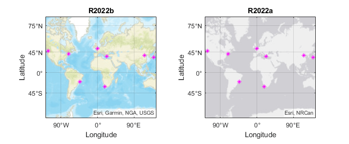
As a result, you can specify a basemap and then visualize data without using the hold function between commands. For example, this code creates a map using the streets basemap. Then it displays a plot over the basemap. In R2022b, the basemap does not reset. In R2022a and earlier releases, the basemap resets to the default streets-light.
lat = [35 -22 51 39 37 42 47 -33];
lon = [139 -43 0 116 23 -71 -122 18];

figure
geobasemap streets
geoplot(lat,lon,"m*")
This change does not affect existing code that sets the hold state to "on" between commands.
To reset the basemap when you add a new plot, use the cla reset syntax of
the cla function before you create the plot.
For example, to update the preceding code, use cla reset between the
calls to geobasemap and geoplot.
lat = [35 -22 51 39 37 42 47 -33];
lon = [139 -43 0 116 23 -71 -122 18];

figure
geobasemap streets
cla reset
geoplot(lat,lon,"m*")
Alternatively, you can change the basemap to the default streets-light by using the geobasemap function. For more information about changing the basemap of geographic axes, see Access Basemaps for Geographic Axes and Charts.
See Also
Functions
geoscatter|geobubble|plot|geobasemap|geoplot(Mapping Toolbox)
Properties
- Line Properties | GeographicAxes Properties | MapAxes Properties (Mapping Toolbox)
1 Alignment of boundaries and region labels are a presentation of the feature provided by the data vendors and do not imply endorsement by MathWorks®.