zpk
Modèle zéro-pôle-gain
Description
Utilisez zpk pour créer des modèles zéro-pôle-gain ou pour convertir des modèles de systèmes dynamiques en modèles zéro-pôle-gain.
Les modèles zéro-pôle-gain représentent les fonctions de transfert sous forme factorisée. Par exemple, considérons la fonction de transfert SISO en temps continu suivante :
G(s) peut être factorisée sous la forme zéro-pôle-gain comme suit :
Une représentation plus générale du modèle SISO zéro-pôle-gain est la suivante :
Ici, z et p sont les vecteurs des zéros et des pôles à valeurs réelles ou complexes, et k est le gain scalaire à valeurs réelles ou complexes. Pour les modèles MIMO, chaque canal d'E/S est représenté par une fonction de transfert de ce type hij(s).
Vous pouvez créer un objet de modèle zéro-pôle-gain en spécifiant directement les pôles, zéros et gains ou en convertissant un modèle d’un autre type (tel qu’un modèle de représentation d’état ss) en modèle zéro-pôle-gain.
Vous pouvez également utiliser zpk pour créer des modèles de représentation d’état généralisés (genss) ou incertains (uss (Robust Control Toolbox)).
Création
Syntaxe
Description
Créer un modèle ZPK
sys = zpk(zeros,poles,gain)zeros et poles spécifiés comme des vecteurs et la valeur scalaire de gain. La sortie sys obtenue est un objet modèle zpk stockant les données du modèle. Réglez zeros ou poles sur [] pour les systèmes sans zéros ni pôles. Ces deux entrées n’ont pas besoin de présenter la même longueur et le modèle n’a pas à être correct (autrement dit avoir un excès de pôles).
sys = zpk(___,PropertyName=Value)
Convertir en modèle ZPK
sys = zpk(ltiSys,Name=Value)zpk tronquée du modèle parcimonieux ltiSys en calculant les zéros et les pôles sur la base d’un ou plusieurs arguments nom-valeur spécifiés. Puisque cette méthode calcule les zéros pour chaque paire d’entrée-sortie, elle convient mieux aux modèles ayant de petites tailles d’entrées-sorties. (depuis R2025a)
Créer une variable pour une expression rationnelle
s = zpk('s') crée une variable spéciale s que vous pouvez utiliser dans une expression rationnelle pour créer un modèle zéro-pôle-gain en temps continu. Il est parfois plus aisé et plus intuitif de recourir à une expression rationnelle plutôt que de spécifier des coefficients polynomiaux.
Arguments en entrée
Arguments nom-valeur
Arguments en sortie
Propriétés
Fonctions d'objet
Les listes suivantes contiennent un sous-ensemble représentatif des fonctions que vous pouvez utiliser avec les modèles zpk. En règle générale, toute fonction applicable à Modèles de systèmes dynamiques est applicable à un objet zpk.
Exemples
Pour les besoins de cet exemple, considérons le modèle SISO zéro-pôle-gain en temps continu suivant :
Spécifiez les zéros, les pôles et le gain, et créez le modèle SISO zéro-pôle-gain.
zeros = 0;
poles = [1-1i 1+1i 2];
gain = -2;
sys = zpk(zeros,poles,gain)
sys =

          -2 s
  --------------------
  (s-2) (s^2 - 2s + 2)

Continuous-time zero/pole/gain model.
Model Properties
Pour cet exemple, considérons le modèle SISO zéro-pôle-gain en temps discret suivant, avec un pas d’échantillonnage de 0,1 s :
Spécifiez les zéros, les pôles et le gain, ainsi que le pas d’échantillonnage, et créez le modèle SISO zéro-pôle-gain en temps discret.
zeros = [1 2 3];
poles = [6 5 4];
gain = 7;
ts = 0.1;
sys = zpk(zeros,poles,gain,ts)
sys =

  7 (z-1) (z-2) (z-3)
  -------------------
   (z-6) (z-5) (z-4)

Sample time: 0.1 seconds
Discrete-time zero/pole/gain model.
Model Properties
Dans cet exemple, vous créez un modèle MIMO zéro-pole-gain en concaténant des modèles SISO zéro-pole-gain. Considérons le modèle zéro-pôle-gain en temps continu à une entrée et deux sorties suivant :
Spécifiez le modèle MIMO zéro-pôle-gain en concaténant les entrées SISO.
zeros1 = 1;
poles1 = -1;
gain = 1;
sys1 = zpk(zeros1,poles1,gain)
sys1 =

  (s-1)
  -----
  (s+1)

Continuous-time zero/pole/gain model.
Model Properties
zeros2 = -2;
poles2 = [-2+1i -2-1i];
sys2 = zpk(zeros2,poles2,gain)
sys2 =

      (s+2)
  --------------
  (s^2 + 4s + 5)

Continuous-time zero/pole/gain model.
Model Properties
sys = [sys1;sys2]
sys =

  From input to output...
       (s-1)
   1:  -----
       (s+1)

           (s+2)
   2:  --------------
       (s^2 + 4s + 5)

Continuous-time zero/pole/gain model.
Model Properties
Créez un modèle zéro-pôle-gain en temps discret, à entrées et sorties multiples :
avec un pas d’échantillonnage de ts = 0.2 secondes.
Spécifiez les zéros et pôles sous la forme de cell arrays et les gains sous la forme d’un tableau.
zeros = {[] 0;2 []};
poles = {-0.3 -0.3;-0.3 -0.3};
gain = [1 1;-1 3];
ts = 0.2;
Créez un modèle MIMO zéro-pôle-gain en temps discret.
sys = zpk(zeros,poles,gain,ts)
sys =

  From input 1 to output...
          1
   1:  -------
       (z+0.3)

       - (z-2)
   2:  -------
       (z+0.3)

  From input 2 to output...
          z
   1:  -------
       (z+0.3)

          3
   2:  -------
       (z+0.3)

Sample time: 0.2 seconds
Discrete-time zero/pole/gain model.
Model Properties
Spécifiez les zéros, pôles et le gain, ainsi que le pas d’échantillonnage et créez le modèle zéro-pôle-gain en spécifiant les noms des noms d’état et d’entrée au moyen de paires nom-valeur.
zeros = 4;
poles = [-1+2i -1-2i];
gain = 3;
ts = 0.05;
sys = zpk(zeros,poles,gain,ts,'InputName','Force')
sys =

  From input "Force" to output:
     3 (z-4)
  --------------
  (z^2 + 2z + 5)

Sample time: 0.05 seconds
Discrete-time zero/pole/gain model.
Model Properties
Le nombre de noms d’entrée doit être cohérent avec le nombre de zéros.
Il peut être utile d’attribuer des noms aux entrées et aux sorties lorsque vous utilisez des tracés de réponse pour les systèmes MIMO.
step(sys)

Notez le nom de l'entrée Force dans le titre du tracé de réponse indicielle.
Pour cet exemple, créez un modèle zéro-pôle-gain en temps continu avec des expressions rationnelles. Il est parfois plus aisé et plus intuitif de recourir à une expression rationnelle plutôt que de spécifier des pôles et des zéros.
Considérons le système suivant :
Pour créer le modèle de fonction de transfert, commencez par spécifier s en tant qu’objet zpk.
s = zpk('s')s = s Continuous-time zero/pole/gain model. Model Properties
Créez le modèle zéro-pôle-gain en utilisant s dans l’expression rationnelle.
sys = s/(s^2 + 2*s + 10)
sys =

         s
  ---------------
  (s^2 + 2s + 10)

Continuous-time zero/pole/gain model.
Model Properties
Pour cet exemple, créez un modèle zéro-pôle-gain en temps discret au moyen d’une expression rationnelle. Il est parfois plus aisé et plus intuitif de recourir à une expression rationnelle plutôt que de spécifier des pôles et des zéros.
Considérons le système suivant :
Pour créer le modèle zéro-pôle-gain, commencez par spécifier z en tant qu’objet zpk et le pas d’échantillonnage ts.
ts = 0.1;
z = zpk('z',ts)
z = z Sample time: 0.1 seconds Discrete-time zero/pole/gain model. Model Properties
Créez le modèle zéro-pôle-gain en utilisant z dans l’expression rationnelle.
sys = (z - 1) / (z^2 - 1.85*z + 0.9)
sys =

         (z-1)
  -------------------
  (z^2 - 1.85z + 0.9)

Sample time: 0.1 seconds
Discrete-time zero/pole/gain model.
Model Properties
Pour cet exemple, créez un modèle zéro-pôle-gain avec les propriétés héritées d’un autre modèle du même type. Considérons les deux modèles zéro-pôle-gain suivants :
Pour cet exemple, créez sys1 en configurant les propriétés TimeUnit et InputDelay en minutes.
zero1 = 0;
pole1 = [0;-8];
gain1 = 2;
sys1 = zpk(zero1,pole1,gain1,'TimeUnit','minutes','InputUnit','minutes')
sys1 =

    2 s
  -------
  s (s+8)

Continuous-time zero/pole/gain model.
Model Properties
propValues1 = [sys1.TimeUnit,sys1.InputUnit]
propValues1 = 1×2 cell
    {'minutes'}    {'minutes'}
Créez le deuxième modèle zéro-pôle-gain avec les propriétés héritées de sys1.
zero = 1;
pole = [-3,5];
gain2 = 0.8;
sys2 = zpk(zero,pole,gain2,sys1)
sys2 =

   0.8 (s-1)
  -----------
  (s+3) (s-5)

Continuous-time zero/pole/gain model.
Model Properties
propValues2 = [sys2.TimeUnit,sys2.InputUnit]
propValues2 = 1×2 cell
    {'minutes'}    {'minutes'}
Comme vous pouvez le constater, le modèle zéro-pôle-gain sys2 comporte les mêmes propriétés que sys1.
Considérons la matrice de gain statique suivante à deux entrées et deux sorties m :
Spécifiez la matrice de gain et créez le modèle zéro-pôle-gain à gain statique.
m = [2,4;...
    3,5];
sys1 = zpk(m)
sys1 = From input 1 to output... 1: 2 2: 3 From input 2 to output... 1: 4 2: 5 Static gain. Model Properties
Vous pouvez utiliser le modèle zéro-pôle-gain à gain statique sys1 obtenu précédemment et l’organiser en cascade avec un autre modèle du même type.
sys2 = zpk(0,[-1 7],1)
sys2 =

       s
  -----------
  (s+1) (s-7)

Continuous-time zero/pole/gain model.
Model Properties
sys = series(sys1,sys2)
sys =

  From input 1 to output...
           2 s
   1:  -----------
       (s+1) (s-7)

           3 s
   2:  -----------
       (s+1) (s-7)

  From input 2 to output...
           4 s
   1:  -----------
       (s+1) (s-7)

           5 s
   2:  -----------
       (s+1) (s-7)

Continuous-time zero/pole/gain model.
Model Properties
Pour cet exemple, calculez le modèle zéro-pôle-gain du modèle de représentation d’état suivant :
Créez le modèle de représentation d’état au moyen des matrices de représentation d’état.
A = [-2 -1;1 -2];
B = [1 1;2 -1];
C = [1 0];
D = [0 1];
ltiSys = ss(A,B,C,D);
Convertissez le modèle de représentation d’état ltiSys en un modèle zéro-pôle-gain.
sys = zpk(ltiSys)
sys =

  From input 1 to output:
        s
  --------------
  (s^2 + 4s + 5)

  From input 2 to output:
  (s^2 + 5s + 8)
  --------------
  (s^2 + 4s + 5)

Continuous-time zero/pole/gain model.
Model Properties
Vous pouvez utiliser une boucle for pour spécifier un tableau de modèles zéro-pôle-gain.
Commencez par pré-attribuer le tableau des modèles zéro-pôle-gain avec des zéros.
sys = zpk(zeros(1,1,3));
Les deux premiers indices représentent le nombre de sorties et d'entrées pour les modèles, tandis que le troisième indice correspond au nombre de modèles figurant dans le tableau.
Créez le tableau de modèles zéro-pôle-gain en utilisant une expression rationnelle dans la boucle for.
s = zpk('s');
for k = 1:3
    sys(:,:,k) = k/(s^2+s+k);
end
sys
sys(:,:,1,1) =

        1
  -------------
  (s^2 + s + 1)


sys(:,:,2,1) =

        2
  -------------
  (s^2 + s + 2)


sys(:,:,3,1) =

        3
  -------------
  (s^2 + s + 3)

3x1 array of continuous-time zero/pole/gain models.
Model Properties
Pour cet exemple, extrayez la composante mesurée et la composante de bruit d’un modèle polynomial identifié vers deux modèles zéro-pôle-gain distincts.
Chargez le modèle polynomial de Box-Jenkins ltiSys dans identifiedModel.mat.
load('identifiedModel.mat','ltiSys');
ltiSys est un modèle identifié en temps discret du type : où représente la composante mesurée et , la composante de bruit.
Extrayez la composante mesurée et la composante de bruit en tant que modèles zéro-pôle-gain.
sysMeas = zpk(ltiSys,'measured') sysMeas =
From input "u1" to output "y1":
-0.14256 z^-1 (1-1.374z^-1)
z^(-2) * -----------------------------
(1-0.8789z^-1) (1-0.6958z^-1)
Sample time: 0.04 seconds
Discrete-time zero/pole/gain model.
Model Properties
sysNoise = zpk(ltiSys,'noise')sysNoise =
From input "v@y1" to output "y1":
0.045563 (1+0.7245z^-1)
--------------------------------------------
(1-0.9658z^-1) (1 - 0.0602z^-1 + 0.2018z^-2)
Input groups:
Name Channels
Noise 1
Sample time: 0.04 seconds
Discrete-time zero/pole/gain model.
Model Properties
La composante mesurée peut servir de modèle de système physique tandis que la composante de bruit peut être utilisée en tant que modèle de perturbations pour le design du système de contrôle.
Pour cet exemple, créez un modèle SISO zéro-pôle-gain avec un retard en entrée de 0,5 seconde et un retard en sortie de 2,5 secondes.
zeros = 5;
poles = [7+1i 7-1i -3];
gains = 1;
sys = zpk(zeros,poles,gains,'InputDelay',0.5,'OutputDelay',2.5)
sys =

                      (s-5)
  exp(-3*s) * ----------------------
              (s+3) (s^2 - 14s + 50)

Continuous-time zero/pole/gain model.
Model Properties
Vous pouvez également utiliser la commande get pour afficher toutes les propriétés d’un objet MATLAB.
get(sys)
                Z: {[5]}
                P: {[3×1 double]}
                K: 1
    DisplayFormat: 'roots'
         Variable: 's'
          IODelay: 0
       InputDelay: 0.5000
      OutputDelay: 2.5000
        InputName: {''}
        InputUnit: {''}
       InputGroup: [1×1 struct]
       OutputName: {''}
       OutputUnit: {''}
      OutputGroup: [1×1 struct]
            Notes: [0×1 string]
         UserData: []
             Name: ''
               Ts: 0
         TimeUnit: 'seconds'
     SamplingGrid: [1×1 struct]
Pour plus d'informations sur la spécification d’un retard pour un modèle LTI, consultez Specifying Time Delays.
Pour cet exemple, concevez un contrôleur PID 2-DOF avec une bande passante cible de 0,75 rad/s pour un système représenté par le modèle zéro-pôle-gain suivant :
Créez un objet modèle zéro-pôle-gain sys au moyen de la commande zpk.
zeros = [];
poles = [-0.25+0.2i;-0.25-0.2i];
gain = 1;
sys = zpk(zeros,poles,gain)
sys =

            1
  ---------------------
  (s^2 + 0.5s + 0.1025)

Continuous-time zero/pole/gain model.
Model Properties
Au moyen de la bande passante cible, utilisez pidtune pour générer un contrôleur 2-DOF.
wc = 0.75;
C2 = pidtune(sys,'PID2',wc)
C2 =
1
u = Kp (b*r-y) + Ki --- (r-y) + Kd*s (c*r-y)
s
with Kp = 0.512, Ki = 0.0975, Kd = 0.574, b = 0.38, c = 0
Continuous-time 2-DOF PID controller in parallel form.
Model Properties
Lorsque le type 'PID2' est utilisé, pidtune génère un contrôleur 2-DOF représenté en tant qu’objet pid2. L’affichage confirme ce résultat. L’affichage indique également que pidtune règle tous les coefficients du contrôleur, y compris les poids des points de consigne b et c, pour équilibrer la performance et la robustesse.
Pour en savoir plus sur le réglage PID interactif dans le Live Editor, voir la tâche Tune PID Controller Live Editor. Cette tâche vous permet de concevoir un contrôleur PID de manière interactive et génère automatiquement un code MATLAB pour votre live script.
Pour effectuer un réglage PID interactif dans une application autonome, utilisez PID Tuner. Pour consulter un exemple de conception d’un contrôleur au moyen de l’application, voir Design d'un contrôleur PID pour le suivi rapide des consignes.
Depuis R2025a
Cet exemple indique comment obtenir un modèle zéro-pôle-gain tronqué d’un modèle de représentation d’état parcimonieux. Cet exemple utilise un modèle parcimonieux obtenu à partir de la linéarisation d’un modèle thermique de distribution de la chaleur dans une tige de vérin circulaire.
Chargez les données du modèle.
load cylindricalRod.mat
sys = sparss(A,B,C,D,E);
w = logspace(-7,-1,20);
size(sys)
Sparse state-space model with 3 outputs, 1 inputs, and 7522 states.
Analysez la réponse en fréquence du modèle.
sigmaplot(sys,w)
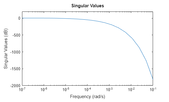
Pour obtenir une approximation tronquée, utilisez zpk et spécifiez la bande de fréquence d’attention. Pour ce modèle, vous pouvez utiliser une plage de fréquence de 0 rad/s à 0,01 rad/s pour obtenir l’approximation d’ordre faible.
zsys = zpk(sys,Focus=[0 1e-2],Display="off");Comparez la réponse en fréquence.
sigmaplot(sys,zsys,w)
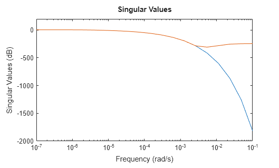
Ce modèle thermique présente une atténuation très abrupte sous 0,001 rad/s. Par défaut, le modèle réduit obtenu au moyen de zpk ne fournit pas de bonne correspondance à cette atténuation. Pour atténuer cela, vous pouvez utiliser l’argument RollOff de zpk et spécifier une valeur d’atténuation minimale au-delà de la bande de fréquence d’attention. Spécifiez une valeur de pente d’atténuation de -45, qui correspond à une vitesse d’au moins –900 dB/décade.
zsys2 = zpk(sys,Focus=[0 1e-2],RollOff=-45,Display="off");
sigmaplot(sys,zsys2,w)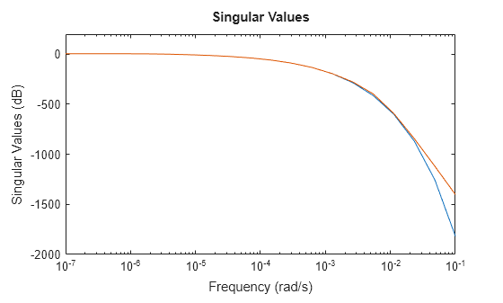
Le modèle réduit fournit maintenant une bien meilleure approximation de la valeur d’atténuation. Cependant, dans cet exemple, réajuster la pente d’atténuation au moyen de zpk nécessite de recalculer les zéros et les pôles. Cela pourrait devenir coûteux en calcul dans le cas de modèles à grande échelle. Comme alternative, vous pouvez utiliser la méthode de troncature zéro-pôle de reducespec et ajuster l’atténuation sans coût de calcul supplémentaire, après que le logiciel a calculé les pôles et les zéros. Pour un exemple, voir Zero-Pole Truncation of Thermal Model.
Algorithmes
zpk utilise la fonction MATLAB roots pour convertir des fonctions de transfert et les fonctions zero et pole pour convertir des modèles de représentation d’état.
Pour convertir des modèles parcimonieux, zpk utilise l’algorithme de Krylov-Schur [1] pour les itérations de puissance inverse pour calculer les pôles et les zéros dans la bande de fréquence.
Références
[1] Stewart, G. W. “A Krylov--Schur Algorithm for Large Eigenproblems.” SIAM Journal on Matrix Analysis and Applications 23, no. 3 (January 2002): 601–14. https://doi.org/10.1137/S0895479800371529.